I have always wanted to approach the problem of wealth distribution from the perspective of Markov processes and related methods, and this is what I will do through the article “Fokker-Planck Description of Wealth Dynamics and the Origin of Pareto’s Law”.

Let us recall that, for a single variable, we obtained the equation

\frac{\partial P(x,t)}{\partial t} = \frac{\partial^{2}}{\partial x^{2}} \left[ D P(x,t) \right] + \frac{\partial}{\partial x} \left[ D\beta \frac{\partial U(x)}{\partial x} P(x,t) \right].

(1)

In this case, we assumed a constant diffusion coefficient,

A=D,

(2)

and a drift term determined by a conservative potential,

B = D\beta \frac{\partial U(x)}{\partial x}.

(3)

More generally, the equation can be written as

\frac{\partial P}{\partial t} = \frac{\partial^{2}}{\partial x^{2}} \left[ A(x)P \right] + \frac{\partial}{\partial x} \left[ B(x)P \right].

(4)

Thus, in one dimension, the temporal evolution of the probability density is determined by the spatial derivatives of two fluxes: a diffusive flux, associated with random fluctuations, and a drift flux, associated with the deterministic tendency imposed by external forces.

When $x$ varies through small stochastic steps $\Delta x$ , we define the diffusion coefficient as

A = \frac{1}{2} \left\langle \Delta x^{2} \right\rangle,

(5)

and the drift coefficient as

B = \left\langle \Delta x \right\rangle.

(6)

In the literature, one typically finds the notation

\dot{P}(\mathbf{r},t) = \frac{1}{2} \nabla^{2} \boldsymbol{D}P - \nabla\cdot \left( \boldsymbol{C}P \right).

(7)

Furthermore, we can write

\dot{P}(\mathbf{r},t) = \nabla\cdot \boldsymbol{A}(\mathbf{r},t) + \nabla\cdot \boldsymbol{B}(\mathbf{r},t),

(8)

that is, the temporal evolution of the probability is given by the divergence of the sum of two fluxes: a diffusive flux and a flux generated by external forces.

Before proceeding, however, we will first seek to understand how this equation is derived.

Fokker-Planck Equation with Small Variation Steps¶

This derivation is based on the work of Professor Heff Moehlis, “Derivation of the Fokker-Planck Equation”.

Let us denote by

\left\{ X(t):t\geq0 \right\}

(9)

a one-dimensional stochastic process with

t_{1}>t_{2}>t_{3},

(10)

that is, the ordering is opposite to the usual notation. If $t_{2}$ represents the present, then $t_{1}$ corresponds to the future and $t_{3}$ to the past.

$P(X_{1},t_{1};X_{2},t_{2})$ is the probability that $X(t_{1})=X_{1}$ and $X(t_{2})=X_{2}$ , that is, the joint probability distribution.
$P(X_{1},t_{1}|X_{2},t_{2})$ is the probability that $X(t_{1})=X_{1}$ given that $X(t_{2})=X_{2}$ , that is, the transition probability.

Therefore,

P(X_{1},t_{1};X_{2},t_{2}) = P(X_{1},t_{1}|X_{2},t_{2}) P(X_{2},t_{2}).

(11)

The joint probability that the system is in state $X_{2}$ at time $t_{2}$ and in state $X_{1}$ at the later time $t_{1}$ is equal to the product of the probability that the system is in $X_{2}$ at time $t_{2}$ and the conditional probability that, given the system is in $X_{2}$ at $t_{2}$ , it evolves to state $X_{1}$ at time $t_{1}$ .

This is the standard relation for joint probabilities,

P(A\cap B)=P(A|B)P(B).

(12)

Let us assume that $X(t)$ is a Markov process:

P(X_{1},t_{1}|X_{2},t_{2};X_{3},t_{3}) = P(X_{1},t_{1}|X_{2},t_{2}).

(13)

That is, the probability that the system transitions to state $X_{1}$ depends only on its immediately preceding state $X_{2}$ . Information about earlier states does not provide any additional information.

For a Markov process, the Chapman-Kolmogorov equation is satisfied:

P(X_{1},t_{1}|X_{3},t_{3}) = \int P(X_{1},t_{1}|X_{2},t_{2}) P(X_{2},t_{2}|X_{3},t_{3}) dX_{2}.

(14)

The Chapman-Kolmogorov equation establishes that the probability of the system evolving from state $X_{3}$ at time $t_{3}$ to state $X_{1}$ at time $t_{1}$ can be obtained by considering all possible intermediate states $X_{2}$ at time $t_{2}$ . For each intermediate state, we multiply the probability of the system evolving from $X_{3}$ to $X_{2}$ by the probability of evolving from $X_{2}$ to $X_{1}$ , and then integrate over all possible values of $X_{2}$ , that is, over all possible intermediate states.

Let us assume that the transition probabilities do not depend on the absolute time, but only on the elapsed time interval. Therefore, for simplicity of notation,

P(X_{1},t_{1}-t_{2}|X_{2}) \equiv P(X_{1},t_{1}|X_{2},t_{2}).

(15)

We can then write

P(Y,t|X) \equiv P(Y,t|X,0),

(16)

that is, we have

X(0)=Y, \qquad X(t)=X.

(17)

Let us begin by considering

\int h(Y) \frac{\partial P(Y,t|X)}{\partial t} dY = I.

(18)

The function $h(Y)$ has a finite interval of support,

Y\in[a,b],

(19)

such that outside this interval,

h(Y)=0.

(20)

This is apparently what is meant by the term ``compact support’’ in the article.

Writing

\frac{\partial P(Y,t|X)}{\partial t} = \lim_{\Delta t\rightarrow0} \frac{ P(Y,t+\Delta t|X) - P(Y,t|X) } {\Delta t},

(21)

and substituting into the integral, while using the Chapman-Kolmogorov equation, we obtain

\begin{align} I &= \lim_{\Delta t\rightarrow0} \int h(Y) \frac{ P(Y,t+\Delta t|X) - P(Y,t|X) } {\Delta t} dY\\ &= \lim_{\Delta t\rightarrow0} \frac{1}{\Delta t} \left[ \int h(Y) P(Y,t+\Delta t|X) dY - \int h(Y) P(Y,t|X) dY \right]\\ &= \lim_{\Delta t\rightarrow0} \frac{1}{\Delta t} \left[ \int h(Y) \left( \int P(Y,\Delta t|Z) P(Z,t|X) dZ \right) dY - \int h(Y) P(Y,t|X) dY \right]. \end{align}

(22)

That is, initially we had only a direct transition from $X$ to $Y$ , separated by a time interval $t+\Delta t$ . By applying the Chapman--Kolmogorov equation, we introduce an intermediate state $Z$ at time $t$ , decomposing the trajectory into two successive transitions. The first describes the evolution from $X$ to $Z$ , whose time interval is $t-0=t$ , whereas the second describes the evolution from $Z$ to $Y$ , whose interval is $(t+\Delta t)-t=\Delta t$ . Since the process is homogeneous in time, the transition probability depends only on the duration of the interval and not on the absolute time at which it occurs. Therefore,

P(Y,t+\Delta t|Z,t) = P(Y,\Delta t|Z).

(23)

Notice that only the second transition is rewritten in this way; the total interval between $X$ and $Y$ remains $t+\Delta t$ .

Since the integral runs over all possible states, the integration variable does not represent a specific state, but only an index that enumerates all possible states. Therefore, we can replace $Y$ by $Z$ (or any other symbol), provided that the replacement is made consistently throughout the entire integral. Thus, we can rewrite the integral over $dY$ as an integral over $dZ$ in the second term:

\begin{align} I &= \lim_{\Delta t\rightarrow0} \frac{1}{\Delta t} \left[ \int h(Y) \left( \int P(Y,\Delta t|Z) P(Z,t|X) dZ \right) dY - \int h(Z) P(Z,t|X) dZ \right] \\ &= \lim_{\Delta t\rightarrow0} \frac{1}{\Delta t} \left[ \int P(Z,t|X) \left( \int h(Y)P(Y,\Delta t|Z)dY - h(Z) \right) dZ \right]. \end{align}

(24)

Now, since

\int_{-\infty}^{+\infty} P(Y,\Delta t|Z)dY=1,

(25)

because there is a $100\%$ probability that the system evolves from state $Z$ to some state (we are integrating over all possible states), and since $h(Z)$ does not depend on $Y$ , we have

h(Z)\int f(Y)dY = \int h(Z)f(Y)dY.

(26)

Therefore,

\begin{align} I &= \lim_{\Delta t\rightarrow0} \frac{1}{\Delta t} \left[ \int P(Z,t|X) \left( \int h(Y)P(Y,\Delta t|Z)dY - \int h(Z)P(Y,\Delta t|Z)dY \right) dZ \right] \\ &= \lim_{\Delta t\rightarrow0} \frac{1}{\Delta t} \left[ \int P(Z,t|X) \int P(Y,\Delta t|Z) \left( h(Y)-h(Z) \right) dYdZ \right]. \end{align}

(27)

We now perform a Taylor expansion of $h(Y)$ around $Z$ :

h(Y) = \sum^{\infty}_{n=0} \frac{h^{(n)}(Z)}{n!} (Y-Z)^{n} = h(Z) + \sum^{\infty}_{n=1} \frac{h^{(n)}(Z)}{n!} (Y-Z)^{n}

(28)

Therefore,

\begin{align} I &= \lim_{\Delta t\rightarrow0} \frac{1}{\Delta t} \left[ \int P(Z,t|X) \int P(Y,\Delta t|Z) \left( h(Z) + \sum^{\infty}_{n=1} \frac{h^{(n)}(Z)}{n!} (Y-Z)^{n} - h(Z) \right) dYdZ \right] \\ &= \int P(Z,t|X) \sum^{\infty}_{n=0} \left[ \frac{1}{n!} \lim_{\Delta t\rightarrow0} \frac{1}{\Delta t} \int P(Y,\Delta t|Z) (Y-Z)^{n} dY \right] h^{(n)}(Z) dZ . \end{align}

(29)

Defining the jump moments as

D^{(n)}(Z) = \frac{1}{n!} \lim_{\Delta t\rightarrow0} \frac{1}{\Delta t} \int (Y-Z)^{n} P(Y,\Delta t|Z) dY ,

(30)

we can understand the idea of a jump by recalling that

X(t+\Delta t)-X(t)=Y-Z .

(31)

Therefore, we obtain

\int h(Y) \frac{\partial P(Y,t|X)}{\partial t} dY = \sum^{\infty}_{n=1} \int P(Z,t|X) D^{(n)} h^{(n)}(Z) dZ .

(32)

Each term of the sum is then

\int P(Z,t|X) D^{(n)} h^{(n)}(Z) dZ = \int F_{n}(Z) h^{(n)}(Z) dZ ,

(33)

where

F_{n}(Z) = P(Z,t|X)D^{(n)} .

(34)

For $n=1$ , applying integration by parts, we choose

u=F_{1}(Z) = P(Z,t|X)D^{(1)} \qquad \left( du=F_{1}^{(1)}dZ \right)

(35)

and

dv=h^{(1)}(Z)dZ \qquad (v=h(Z)).

(36)

\int u\,dv=uv-\int v\,du ,

(37)

we have

\int^{+\infty}_{-\infty} F_{1}(Z)h^{(1)}(Z)dZ = \left[ h(Z)F_{1}(Z) \right]^{+\infty}_{-\infty} - \int^{+\infty}_{-\infty} h(Z)F^{(1)}_{1}dZ .

(38)

Since the test function $h(Z)$ has compact support, the boundary term vanishes, because it is zero outside the region of interest. Therefore, we are left with

\int^{+\infty}_{-\infty} F_{1}(Z)h^{(1)}(Z)dZ = - \int^{+\infty}_{-\infty} h(Z)F^{(1)}_{1}dZ .

(39)

For $n=2$ , applying integration by parts once more, we choose

u=F_{2}(Z) = P(Z,t|X)D^{(2)} \qquad \left( du=F^{(1)}_{2}dZ \right)

(40)

and

dv=h^{(2)}(Z)dZ \qquad \left( v=h^{(1)}(Z) \right).

(41)

Therefore,

\int^{+\infty}_{-\infty} F_{2}(Z)h^{(2)}(Z)dZ = - \int^{+\infty}_{-\infty} h^{(1)}(Z)F^{(1)}_{2}dZ .

(42)

Again, due to the fact that $h(Z)$ has compact support, we have that $h^{(1)}(Z)=0$ outside its support, that is, at the boundaries of the integration domain. Performing another integration by parts, with

u=F^{(1)}_{2} = P(Z,t|X)D^{(2)} \qquad \left( du=F^{(2)}_{2}dZ \right)

(43)

and

dv=h^{(1)}(Z)dZ \qquad \left( v=h(Z) \right),

(44)

we obtain

\int^{+\infty}_{-\infty} F_{2}(Z)h^{(2)}(Z)dZ = \int^{+\infty}_{-\infty} h(Z)F^{(2)}_{2}dZ .

(45)

Therefore, in general,

\int F_{n}(Z)h^{(n)}(Z)dZ = (-1)^{n} \int h(Z)F^{(n)}_{n}dZ

(46)

or equivalently,

\int F_{n}(Z)h^{(n)}(Z)dZ = \int h(Z) \left( -\frac{\partial}{\partial Z} \right)^{n} P(Z,t|X)D^{(n)} dZ .

(47)

Therefore,

\int h(Y) \frac{\partial P(Y,t|X)}{\partial t} dY = \sum^{\infty}_{n=1} \int P(Z,t|X) D^{(n)} h^{(n)}(Z) dZ = \int h(Z) \sum^{\infty}_{n=1} \left( -\frac{\partial}{\partial Z} \right)^{n} D^{(n)} P(Z,t|X) dZ .

(48)

Moving the left-hand side to the right and again using $Y\rightarrow Z$ on the left:

\int h(Z) \frac{\partial P(Z,t|X)}{\partial t} dZ - \int h(Z) \sum^{\infty}_{n=1} \left( -\frac{\partial}{\partial Z} \right)^{n} D^{(n)} P(Z,t|X) dZ = 0

(49)

or

\int h(Z) \left( \frac{\partial P(Z,t|X)}{\partial t} - \sum^{\infty}_{n=1} \left( -\frac{\partial}{\partial Z} \right)^{n} D^{(n)} P(Z,t|X) \right) dZ = 0 .

(50)

Since $h(Z)$ is an arbitrary function, in order for this integral to vanish, we must have

\frac{\partial P(Z,t|X)}{\partial t} - \sum^{\infty}_{n=1} \left( -\frac{\partial}{\partial Z} \right)^{n} D^{(n)} P(Z,t|X) = 0 .

(51)

Writing

P(X,t) \equiv P(X,t|X_{0},0),

(52)

that is, this is the probability density of finding the system in state $X$ at time $t$ , given that it was in state $X_{0}$ at time 0. Therefore,

\frac{\partial P(X,t)}{\partial t} - \sum^{\infty}_{n=1} \left( -\frac{\partial}{\partial X} \right)^{n} D^{(n)} P(X,t) = 0 .

(53)

Considering a delta distribution as the initial condition at $X_{0}$ , the probability of obtaining $X$ at the initial time is

P(X,0)=\delta(X-X_{0}),

(54)

which means that, at the initial instant, the random variable $X$ assumes the value $X_{0}$ with unit probability. The entire probability distribution is concentrated at $X_{0}$ , being represented by the Dirac delta distribution.

Therefore, for $D^{(n)}$ :

D^{(n)}(Z) = \frac{1}{n!} \lim_{\Delta t\rightarrow0} \frac{1}{\Delta t} \int (Y-Z)^{n} P(Y,\Delta t|Z) dY

(55)

For $Z=X_{0}$ , we have

\begin{align} D^{(n)}(X_{0}) &= \frac{1}{n!} \lim_{\Delta t\rightarrow0} \frac{1}{\Delta t} \int (X-X_{0})^{n} P(X,\Delta t|X_{0}) dX \\ &= \frac{1}{n!} \lim_{\Delta t\rightarrow0} \frac{1}{\Delta t} \int (\Delta X)^{n} P(X,\Delta t|X_{0}) dX . \end{align}

(56)

Using the definition of expectation values,

D^{(n)}(X_{0}) = \frac{1}{n!} \lim_{\Delta t\rightarrow0} \frac{ \left\langle (\Delta X)^{n} \right\rangle } {\Delta t}.

(57)

Here, $\left\langle(\Delta X)^{n}\right\rangle$ represents the expected value of $(\Delta X)^{n}$ , with

\Delta X=X(\Delta t)-X_{0}(0),

(58)

calculated with respect to the transition probability distribution, that is, considering all possible transitions from the state $X_{0}$ at time 0 to the states $X$ at time $\Delta t$ .

Considering that

D^{(n)}(X)=0 \qquad \text{for} \qquad n>2,

(59)

we obtain

\frac{\partial P(X,t)}{\partial t} + \frac{\partial}{\partial X} \left[ D^{(1)}P(X,t) \right] - \left( \frac{\partial}{\partial X} \right)^{2} D^{(2)}P(X,t) = 0 .

(60)

For $n=1$ and $n=2$ :

D^{(1)}(X_{0}) = \lim_{\Delta t\rightarrow0} \frac{ \left\langle \Delta X \right\rangle } {\Delta t}, \qquad D^{(2)}(X_{0}) = \frac{1}{2} \lim_{\Delta t\rightarrow0} \frac{ \left\langle (\Delta X)^{2} \right\rangle } {\Delta t}.

(61)

Therefore,

\begin{align} \frac{\partial P(X,t)}{\partial t} &= -\frac{\partial}{\partial X} \left[ \lim_{\Delta t\rightarrow0} \frac{ \left\langle \Delta X \right\rangle } {\Delta t} P(X,t) \right] + \frac{\partial^{2}}{\partial X^{2}} \left[ \frac{1}{2} \lim_{\Delta t\rightarrow0} \frac{ \left\langle (\Delta X)^{2} \right\rangle } {\Delta t} P(X,t) \right] \\ &= -\frac{\partial}{\partial X} \left[ V(X)P(X,t) \right] + \frac{\partial^{2}}{\partial X^{2}} \left[ D(X)P(X,t) \right]. \end{align}

(62)

The first term,

V(X)\equiv D^{(1)}(X),

(63)

is the drift coefficient. It is given by

D^{(1)}(X_{0}) = \lim_{\Delta t\rightarrow0} \frac{ \left\langle \Delta X \right\rangle } {\Delta t} = \left. \lim_{\Delta t\rightarrow0} \frac{ \left\langle X(t+\Delta t) \right\rangle - \left\langle X(t) \right\rangle } {\Delta t} \right|_{t=0} = \left. \frac{\partial\left\langle X\right\rangle}{\partial t} \right|_{t=0}.

(64)

The coefficient

D(X)\equiv D^{(2)}(X)

(65)

is the diffusion coefficient.

Recalling that

\begin{array}{c} \left. \left\langle \Delta X \right\rangle \right|_{t=0} = \left. \left( \left\langle X(t+\Delta t) \right\rangle - \left\langle X(t) \right\rangle \right) \right|_{t=0} = \left\langle X(\Delta t) \right\rangle - \left\langle X(0) \right\rangle = \left\langle X(\Delta t) \right\rangle - \left\langle X_{0} \right\rangle \\[10pt] \left. X(\Delta t) \right|_{t=0} = \left. \Delta X \right|_{t=0} + X_{0} \end{array}

(66)

Since $\left\langle X_{0}\right\rangle=X_{0}$ is a constant, by convention we will no longer explicitly indicate that we are evaluating at $t=0$ , although this should be understood.

If the variance at time $t$ , with $X_{0}$ as the initial state, is given by

\begin{align} \sigma^{2}(\Delta t;X_{0}) &= \left\langle X(\Delta t)^{2} \right\rangle - \left\langle X(\Delta t) \right\rangle^{2} \\ &= \left\langle (\Delta X+X_{0})^{2} \right\rangle - \left\langle \Delta X+X_{0} \right\rangle^{2} \\ &= \left\langle \Delta X^{2} + X_{0}^{2} + 2X_{0}\Delta X \right\rangle - \left( X_{0} + \left\langle \Delta X \right\rangle \right)^{2} \\ &= \left\langle \Delta X^{2} \right\rangle + X_{0}^{2} + 2X_{0} \left\langle \Delta X \right\rangle - \left( \left\langle \Delta X \right\rangle^{2} + X_{0}^{2} + 2X_{0} \left\langle \Delta X \right\rangle \right) \\ &= \left\langle \Delta X^{2} \right\rangle - \left\langle \Delta X \right\rangle^{2}. \end{align}

(67)

Therefore,

\left\langle \Delta X^{2} \right\rangle = \sigma^{2}(\Delta t;X_{0}) + \left\langle \Delta X \right\rangle^{2}.

(68)

Thus,

\begin{align} D^{(2)}(X_{0}) &= \frac{1}{2} \lim_{\Delta t\rightarrow0} \frac{ \left\langle (\Delta X)^{2} \right\rangle } {\Delta t} \\ &= \frac{1}{2} \lim_{\Delta t\rightarrow0} \frac{ \sigma^{2}(\Delta t;X_{0}) + \left\langle \Delta X \right\rangle^{2} } {\Delta t} \\ &= \frac{1}{2} \lim_{\Delta t\rightarrow0} \frac{ \sigma^{2}(\Delta t;X_{0}) } {\Delta t} + \frac{1}{2} \lim_{\Delta t\rightarrow0} \frac{ \left\langle \Delta X \right\rangle^{2} } {\Delta t}. \end{align}

(69)

Now, regarding the first moment, we had:

D^{(1)}(X_{0})=\lim_{\Delta t\rightarrow0}\frac{\langle\Delta X\rangle}{\Delta t}.

(70)

For a sufficiently small time interval, we can approximate:

D^{(1)}(X_{0})\approx\frac{\langle\Delta X\rangle}{\Delta t},

(71)

or, equivalently,

\langle\Delta X\rangle\approx D^{(1)}(X_{0})\Delta t.

(72)

Therefore, for the second term:

\lim_{\Delta t\rightarrow0}\frac{\left\langle \Delta X\right\rangle ^{2}}{\Delta t} = \lim_{\Delta t\rightarrow0} \frac{\left[D^{(1)}(X_{0})\right]^{2}\Delta t^{2}}{\Delta t} = \lim_{\Delta t\rightarrow0} \left[D^{(1)}(X_{0})\right]^{2}\Delta t = \left[D^{(1)}(X_{0})\right]^{2} \lim_{\Delta t\rightarrow0}\Delta t =0.

(73)

Now, only the first term remains. If:

\left.\frac{\partial\sigma^{2}}{\partial t}\right|_{t=0} = \left. \lim_{\Delta t\rightarrow0} \frac{\sigma^{2}\left(t+\Delta t;X_{0}\right)-\sigma^{2}\left(t;X_{0}\right)} {\Delta t} \right|_{t=0} = \lim_{\Delta t\rightarrow0} \frac{\sigma^{2}\left(\Delta t;X_{0}\right)-\sigma^{2}\left(0;X_{0}\right)} {\Delta t} = \lim_{\Delta t\rightarrow0} \frac{\sigma^{2}\left(\Delta t;X_{0}\right)} {\Delta t}.

(74)

Since the variance at the initial instant is zero,

\sigma^{2}\left(0;X_{0}\right)=0,

(75)

that is, the value is known exactly. Therefore:

D^{(2)}\left(X_{0}\right) = \frac{1}{2} \left. \frac{\partial\sigma^{2}}{\partial t} \right|_{t=0}.

(76)

Therefore, we have:

\frac{\partial P\left(X,t\right)}{\partial t} = -\frac{\partial}{\partial X} \left[V\left(X\right)P\left(X,t\right)\right] + \frac{\partial^{2}}{\partial X^{2}} \left[D\left(X\right)P\left(X,t\right)\right].

(77)

With:

V\left(X_{0}\right) = \left. \frac{\partial\left\langle X\left(t;X_{0}\right)\right\rangle} {\partial t} \right|_{t=0} \qquad D\left(X_{0}\right) = D^{(2)}\left(X_{0}\right) = \frac{1}{2} \left. \frac{\partial\sigma\left(t;X_{0}\right)^{2}} {\partial t} \right|_{t=0}.

(78)

The Yard-Sale Model¶

Therefore, by setting ( $x=w$ ), we obtain the equation used in the article:

\frac{\partial P}{\partial t} = -\frac{\partial}{\partial w} \left[ \lim_{\Delta t\rightarrow0} \frac{\left\langle \Delta w\right\rangle}{\Delta t}P \right] + \frac{\partial^{2}}{\partial w^{2}} \left[ \frac{1}{2} \lim_{\Delta t\rightarrow0} \frac{\left\langle \Delta w\Delta w\right\rangle}{\Delta t}P \right].

(79)

In the article, we have:

\frac{\partial P}{\partial t} = -\frac{\partial}{\partial w} \left[ \left\langle \Delta(w)\right\rangle P \right] + \frac{\partial^{2}}{\partial w^{2}} \left[ \frac{1}{2} \left\langle \Delta(w)\Delta(w)\right\rangle P \right].

(80)

Therefore:

\left\langle \Delta(w)\right\rangle = \lim_{\Delta t\rightarrow0} \frac{\left\langle \Delta w\right\rangle}{\Delta t} \qquad \left\langle \Delta(w)^{2}\right\rangle = \lim_{\Delta t\rightarrow0} \frac{\left\langle \left(\Delta w\right)^{2}\right\rangle}{\Delta t}.

(81)

To demonstrate this relation, we introduce some additional assumptions. Consider a single realization of the process during a time interval ( $\Delta t$ ), in which ( $\Delta N$ ) transactions occur and the total transferred wealth is ( $\Delta w$ ). We define the average wealth transferred per transaction in this realization as

\left\langle \Delta(w)_{1}\right\rangle \equiv \frac{\Delta w}{\Delta N},

(82)

from which it immediately follows that

\Delta w = \Delta N\left\langle \Delta(w)_{1}\right\rangle .

(83)

Next, we generalize to an ensemble of realizations, in which both ( $\Delta w$ ) and ( $\Delta N$ ) may vary. Taking the mathematical expectation over this ensemble and assuming that the number of transactions occurring within an interval is statistically independent of the average wealth transferred per transaction, we obtain:

The change in notation

\left\langle \Delta(w)_{1}\right\rangle \rightarrow \left\langle \Delta(w)\right\rangle

(84)

indicates that the average is no longer taken within a single realization, but rather over the ensemble.

We have:

\left\langle \Delta w\right\rangle =\left\langle \Delta N\right\rangle \left\langle \Delta(w)\right\rangle .

(85)

For a Poisson process, we assume that the probability of an event occurring within a small time interval is proportional to the time interval. That is,

\left\langle \Delta N\right\rangle =\lambda\Delta t,

(86)

where the larger the time interval, the higher the probability that an exchange occurs.

Therefore,

\left\langle \Delta w\right\rangle = \left\langle \Delta N\right\rangle \left\langle \Delta(w)\right\rangle

(87)

\left\langle \Delta w\right\rangle = \lambda\Delta t\left\langle \Delta(w)\right\rangle

(88)

\frac{\left\langle \Delta w\right\rangle}{\Delta t} = \lambda\left\langle \Delta(w)\right\rangle .

(89)

We will then choose the time unit such that the average time between transactions is one. In this scale, the transaction rate is $\lambda=1$ , so that

\left\langle \Delta N\right\rangle =\Delta t,

(90)

that is, there is on average one transaction per unit of time. Therefore:

\frac{\left\langle \Delta w\right\rangle}{\Delta t} = \left\langle \Delta(w)\right\rangle \rightarrow \lim_{\Delta t\rightarrow0} \frac{\left\langle \Delta w\right\rangle}{\Delta t} = \left\langle \Delta(w)\right\rangle .

(91)

Since the right-hand side does not depend on $\Delta t$ . An analogous reasoning applies to

\left\langle \Delta(w)^{2}\right\rangle .

(92)

However, let us take a step back and consider

\left\langle \Delta(w)_{1}\right\rangle \equiv \frac{\Delta w}{\Delta N},

(93)

while reinforcing the assumption that we are working with a Poisson process. Consider a single realization of the process during a time interval $\Delta t$ , in which $\Delta N$ transactions occur:

\Delta w=\sum^{\Delta N}_{i=1}\Delta(w)_{i}

(94)

\left(\Delta w\right)^{2} = \sum^{\Delta N}_{i,j=1} \Delta(w)_{i}\Delta(w)_{j} = \sum^{\Delta N}_{i=1} \Delta(w)^{2}_{i} + \left( \sum^{\Delta N}_{i\neq j} \Delta(w)_{j}\Delta(w)_{i} \right)

(95)

Taking the average, we obtain:

\left\langle \left(\Delta w\right)^{2}\right\rangle = \left\langle \Delta N\right\rangle \left\langle \Delta(w)^{2}_{E}\right\rangle + \left\langle \sum^{\Delta N}_{i\neq j} \Delta(w)_{j}\Delta(w)_{i} \right\rangle .

(96)

For the first term, we repeat the reasoning from the previous case. Since we avoid the case where $i=j$ , if the first summation involves $\Delta N$ terms, the second sums over $\Delta N$ values for $i$ and $\Delta N-1$ values for $j$ (for example), thereby excluding instances where $i=j$ . Thus, the second summation consists of $\Delta N(\Delta N-1)$ terms. Denoting the ensemble average of the terms $\langle \Delta(w)_j \Delta(w)_i \rangle$ as $\langle \Delta\Delta(w)_E \rangle$ , we write:

\left\langle \left(\Delta w\right)^{2} \right\rangle = \left\langle \Delta N\right\rangle \left\langle \Delta(w)^{2}_{E} \right\rangle + \left\langle \Delta N(\Delta N-1) \right\rangle \left\langle \Delta\Delta(w)_{E} \right\rangle .

(97)

However, now

\left\langle \Delta N(\Delta N-1) \right\rangle

(98)

is slightly more complicated than

\left\langle\Delta N\right\rangle=\lambda\Delta t.

(99)

For now, we will use the factorial moment of the Poisson distribution ([Wikipedia]). Using the notation

(x)_{n} = x(x-1)(x-2)\dots(x-n+1),

(100)

we have:

(N)_{1} = (N-1+1) = N

(101)

and

(N)_{2} = N(N-2+1) = N(N-1).

(102)

For a Poisson distribution, we have

\left\langle (X)_{n} \right\rangle = \mu^{n},

(103)

for a Poisson random variable with mean $\mu$ . Therefore:

\left\langle N\right\rangle = \lambda\Delta t

(104)

and

\left\langle N(N-1) \right\rangle = (\lambda\Delta t)^{2}.

(105)

Thus:

\left\langle \left(\Delta w\right)^{2} \right\rangle = \lambda\Delta t \left\langle \Delta(w)^{2}_{E} \right\rangle + (\lambda\Delta t)^{2} \left\langle \Delta\Delta(w)_{E} \right\rangle .

(106)

Therefore,

\lim_{\Delta t\rightarrow0} \frac{ \left\langle \left(\Delta w\right)^{2} \right\rangle }{\Delta t} = \lambda \left\langle \Delta(w)^{2}_{E} \right\rangle + \lim_{\Delta t\rightarrow0} \lambda\Delta t \left\langle \Delta\Delta(w)_{E} \right\rangle .

(107)

Finally,

\lim_{\Delta t\rightarrow0} \frac{ \left\langle \left(\Delta w\right)^{2} \right\rangle }{\Delta t} = \lambda \left\langle \Delta(w)^{2}_{E} \right\rangle .

(108)

Therefore, since the second term is proportional to $(\Delta t)^{2}$ , after dividing by $\Delta t$ it remains of order $\Delta t$ , vanishing in the continuous limit. This shows that the second Kramers-Moyal coefficient is determined only by the second moment of the wealth transferred in a single transaction, in complete analogy with the result obtained for the first moment. Choosing the time unit as the average interval between transactions, that is, $\lambda=1$ , we obtain

\left\langle \Delta(w)^{2}\right\rangle = \lim_{\Delta t\rightarrow0} \frac{\left\langle \left(\Delta w\right)^{2}\right\rangle}{\Delta t}.

(109)

However, let us pause for a moment and start from the beginning. Suppose that wealth is distributed according to a probability density function (PDF) $P(w)$ . Then,

\int_{a}^{b}P(w)dw

(110)

represents the total population of agents with wealth $w\in[a,b]$ , and the fraction of the population with wealth greater than $w$ is given by

A(w)= \frac{\int_{w}^{\infty}P(w')dw'} {\int_{0}^{\infty}P(w)dw}.

(111)

Pareto found the following approximation:

A_{p}(w)= \begin{cases} 1, & w< w_{min}\\ \left(\frac{w_{min}}{w}\right)^{\alpha}, & w\geq w_{min}. \end{cases}

(112)

Before proceeding, it seems interesting to make one more observation. In the description of the model, it is assumed that the commodity possesses an “intrinsic value”, and that when agents exchange with each other, they assign a price different from this intrinsic value, that is, they evaluate it above or below its intrinsic value. This causes a transfer of wealth (measured in intrinsic value) between agents.

In this description, the concept of the agent’s “utility function” is even mentioned to justify this incorrect valuation (it is worth noting that this is explicitly described as an error). It is interesting that, while attempting to preserve the idea of a utility function from marginalist microeconomics, the model simultaneously postulates the existence of an objective value that differs from the price.

However, continuing, we aim to model the exchange of wealth between two agents such that:

One agent has wealth $w$ and another has wealth $w'$ .
The amount to be transferred is a fraction $\beta$ of the wealth of the poorer agent.
- The amount of wealth being transferred from $w'$ to $w$ is
  $\Delta(w,w',r)=\beta r\min(w,w').$
  (113)
The beneficiary of the exchange is either one of the two agents with equal probability.
- That is, $r=\pm1$ with equal probability.

After the transaction, the wealth of the agents is:

w_{final}=w+\Delta(w,w',r)

(114)

w'_{final}=w'-\Delta(w,w',r).

(115)

Using a Heaviside step function,

\theta(x) = \begin{cases} 1, & x\geq0\\ 0, & x< 0 \end{cases},

(116)

we can write:

\Delta(w,w',r) = \beta r \left[ w\theta(w'-w) + w'\theta(w-w') \right].

(117)

That is, if $w'< w$ , only the second term remains, and we have a fraction of $w'$ being transferred. Conversely, if $w< w'$ , only the first term remains.

But what happens when $w'=w$ ? In this case, the expression gives twice the value, which may be problematic. For example, if $w=w'=1$ and $\beta=r=1$ , then

\Delta(w,w',r)=2.

(118)

This would imply

w'_{final}=-1,

(119)

which is not physically meaningful.

I believe this issue will not affect the equations developed later, since they deal with probability flows. However, a simple way to resolve it is to use another popular definition of the Heaviside function:

\theta(x) = \begin{cases} 1, & x>0\\ \frac{1}{2}, & x=0\\ 0, & x< 0 \end{cases}.

(120)

With this definition, we can now return to the Fokker-Planck equation:

\frac{\partial P}{\partial t} = -\frac{\partial}{\partial w} \left[ \left\langle \Delta(w)\right\rangle P \right] + \frac{\partial^{2}}{\partial w^{2}} \left[ \frac{1}{2} \left\langle \Delta(w)\Delta(w)\right\rangle P \right].

(121)

Here, $\left\langle .\right\rangle$ denotes the average over the distribution of step sizes, that is, in this case, the average over the distribution of possible amounts of wealth transferred in an interaction.

The wealth variation of an agent with wealth $w$ after a transaction has two sources of stochasticity:

The wealth $w'$ of the partner agent must be obtained from a sample of the probability distribution function $P(w')$ .
The random variable $r$ .

We define the average of the function $f(w',r)$ over these two sources of randomness as:

\left\langle f\right\rangle = \frac{1}{N} \int dw'P(w') \frac{f(w',-1)+f(w',+1)}{2}.

(122)

Since $P(w)$ is not normalized, $\frac{P(w')}{N}$ is only the normalized probability density function. Therefore,

\left\langle f\right\rangle = \int \left[ \frac{f(w',-1)+f(w',+1)}{2} \right] \left[ \frac{P(w')}{N} \right] dw'.

(123)

Now we need to understand why we are calculating the average over the first term inside the brackets. We want an average over both sources of randomness. For a fixed value of $w'$ , there are two possible values of $r$ with equal probability. Therefore,

\left\langle f\right\rangle_{r} = \frac{f(w',-1)+f(w',+1)}{2}.

(124)

Now, if we calculate the average of $\left\langle f\right\rangle_{r}$ over all possible values of $w'$ , we are applying the Law of Total Expectation:

E[f]=E_{w'}\left[E_{r}(f(w',r)|w')\right].

(125)

This means that the global average of $f$ (over both sources of randomness) is calculated in two steps: (i) we fix the partner’s wealth $w'$ and calculate the average over the variable $r$ ; (ii) we then average these results over all possible values of the partner’s wealth $w'$ , weighted by their probability of occurrence.

It is worth noting that $E_i[f]$ indicates that the average is taken over the variable $i$ . Therefore,

\left\langle f\right\rangle = \int \left\langle f\right\rangle_{r} \left[ \frac{P(w')}{N} \right] dw'

(126)

or equivalently,

\left\langle f\right\rangle = \int \frac{f(w',-1)+f(w',+1)}{2} \frac{P(w')}{N} dw'.

(127)

Taking

f=\Delta(w),

(128)

we obtain:

\left\langle \Delta(w)\right\rangle = \int \frac{ \Delta(w,w',-1)+\Delta(w,w',+1) }{2} \frac{P(w')}{N} dw'.

(129)

It is worth noting that, for any pair $(w,w')$ ,

\Delta(w,w',-1)+\Delta(w,w',+1) = -\beta\min(w,w') + \beta\min(w,w') = 0.

(130)

Therefore,

\left\langle \Delta(w)\right\rangle =0.

(131)

Now, taking

f=\Delta(w)^{2},

(132)

we obtain:

\left\langle \Delta(w)^{2}\right\rangle = \int \frac{ \Delta(w,w',-1)^{2} + \Delta(w,w',+1)^{2} }{2} \frac{P(w')}{N} dw'.

(133)

Therefore, defining

S= \Delta(w,w',-1)^{2} + \Delta(w,w',+1)^{2},

(134)

we have

S= \left( -\beta \left[ w\theta(w'-w) + w'\theta(w-w') \right] \right)^{2} + \left( \beta \left[ w\theta(w'-w) + w'\theta(w-w') \right] \right)^{2},

(135)

which gives

S= 2\beta^{2} \left[ w\theta(w'-w) + w'\theta(w-w') \right]^{2}.

(136)

Using the definition

\theta(x) = \begin{cases} 1, & x\geq0\\ 0, & x< 0 \end{cases},

(137)

we have that

\theta(w'-w)\theta(w-w')=0

(138)

for $w'\neq w$ , since one of the two factors is always zero. The cross term survives only when $w=w'$ , namely,

2ww'\theta(w'-w)\theta(w-w').

(139)

However, this case corresponds to a single point in the integration domain. Since a set composed of a single point has null measure, its contribution to the integral is zero. In one dimension, the measure of a set corresponds to its length; in two dimensions, to its area; in three dimensions, to its volume. More generally, integrals are computed with respect to the measure of the integration domain.

Furthermore, since

\theta(x)=\theta^{2}(x),

(140)

we obtain:

S= 2\beta^{2} \left[ w^{2}\theta(w'-w) + w'^{2}\theta(w-w') \right].

(141)

Substituting into the expression for the second moment, we obtain:

\left\langle \Delta(w)^{2}\right\rangle = \int \frac{ 2\beta^{2} \left[ w^{2}\theta(w'-w) + w'^{2}\theta(w-w') \right] }{2} \frac{P(w')}{N} dw'.

(142)

Since the first term contributes only for $w'<\infty$ with $w'>w$ , and the second term only for $w'<w$ , we have:

\left\langle \Delta(w)^{2}\right\rangle = \beta^{2} \left( \int_{w}^{\infty} w^{2} \frac{P(w')}{N} dw' + \int_{0}^{w} w'^{2} \frac{P(w')}{N} dw' \right).

(143)

Rewriting the first term using the definition of $A(w)$ ,

A(w) = \frac{ \int_{w}^{\infty}P(w')dw' }{ \int_{0}^{\infty}P(w)dw },

(144)

and defining

B(w) = \frac{1}{2} \int_{0}^{w} w'^{2} \frac{P(w')}{N} dw',

(145)

we obtain:

\left\langle \Delta(w)^{2}\right\rangle = \beta^{2} 2 \left( \frac{w^{2}}{2}A(w) + B(w) \right).

(146)

where the first term is the Pareto function defined previously. We can therefore write the Fokker-Planck equation as:

\frac{\partial P}{\partial t} = -\frac{\partial}{\partial w} \left[ \left\langle \Delta(w)\right\rangle P \right] + \frac{\partial^{2}}{\partial w^{2}} \left[ \frac{1}{2} \left\langle \Delta(w)\Delta(w) \right\rangle P \right]

(147)

= \frac{\partial^{2}}{\partial w^{2}} \left[ \frac{1}{2} \left( \beta^{2}2 \left( \frac{w^{2}}{2}A(w)+B(w) \right) \right) P \right]

(148)

= \beta^{2} \frac{\partial^{2}}{\partial w^{2}} \left[ \left( \frac{w^{2}}{2}A+B \right) P \right].

(149)

We can also show the conservation of the population by integrating the left-hand side:

\frac{\partial}{\partial t}\int P\,dw = \frac{\partial N}{\partial t} = \dot{N} = 0,

(150)

and the conservation of wealth:

\frac{\partial}{\partial t}\int wP\,dw = \frac{\partial W}{\partial t} = \dot{W} = 0.

(151)

Writing

\frac{\partial P}{\partial t} = \frac{\partial^{2}F(w)}{\partial w^{2}} = F''(w),

(152)

where

F(w) = \beta^{2} \left( \frac{w^{2}}{2}A+B \right) P,

(153)

we have

\dot{N} = \int_{0}^{+\infty} F''(w)\,dw = F'(\infty)-F'(0).

(154)

Defining

J(w)=-F'(w),

(155)

we identify $J(w)$ as the probability flux:

\frac{\partial P}{\partial t} = \frac{\partial^{2}F(w)}{\partial w^{2}} = -\frac{\partial J}{\partial w}.

(156)

Therefore, assuming a vanishing net probability flux between the boundaries, we have

0 = F'(\infty)-F'(0) = \dot{N}.

(157)

For $\dot{W}$ , we need to use integration by parts, taking

u=w, \qquad du=dw,

(158)

and

dv=F''(w)dw, \qquad v=F'(w).

(159)

\dot{W} = \int_{0}^{+\infty} wF''(w)dw = \left[wF'(w)\right]_{0}^{+\infty} - \int_{0}^{+\infty}F'(w)dw.

(160)

The second integral has already been shown to be zero. Therefore,

\dot{W} = \lim_{w\rightarrow\infty}wF'(w) - \lim_{w\rightarrow0}wF'(w).

(161)

Lower boundary ( $w\rightarrow0$ ): $\lim_{w\rightarrow0}wF'(w)$ .

Calculating $F'(w)$ explicitly, we have:

F' = \beta^{2} \left[ \left( wA+\frac{w^{2}}{2}A'+B' \right)P + \left( \frac{w^{2}}{2}A+B \right)P' \right].

(162)

Taking $N=1$ , we have

A' = \left[ \int_{w}^{\infty}P(w')dw' \right]' = -P(w),

(163)

since $P(w)$ must vanish at infinity, and

B'(w) = \frac{1}{2} \left[ \int_{0}^{w}w'^{2}P(w')dw' \right]' = \frac{w^{2}}{2}P(w),

(164)

where we have assumed that $P(0)$ has a finite value at $w=0$ .

Therefore, for $w\rightarrow0$ ,

F'(0) = \beta^{2} \left[ \left( 0+0+0 \right)P(0) + \left( 0+0 \right)P'(0) \right] = 0.

(165)

Therefore,

\lim_{w\rightarrow0}wF'(w)=0,

(166)

provided that $P(0)$ and $P'(0)$ do not diverge too rapidly. Since $B(0)=0$ trivially, it is sufficient that $P(0)$ remains finite, which is a reasonable condition.

Upper boundary ( $w\rightarrow\infty$ )

Writing

F'(w) = \beta^{2} \left[ \left( w\int_{w}^{\infty}P(w')dw' -\frac{w^{2}}{2}P(w) +\frac{w^{2}}{2}P(w) \right)P(w) + \left( \frac{w^{2}}{2} \int_{w}^{\infty}P(w')dw' + \int_{0}^{w}\frac{w'^{2}}{2}P(w')dw' \right) P'(w) \right].

(167)

For

\lim_{w\rightarrow\infty}wF'(w)=0,

(168)

it is necessary and sufficient that the tail of the distribution $P(w)$ and its derivative $P'(w)$ decay sufficiently fast. This is again a reasonable assumption, since no agent can possess infinite wealth.

Moreover, for $A(\infty)=0$ , we now have a trivial integral, since the integration limits are identical.

In summary, we assume the following regularity conditions:

$P(w)$ is differentiable in a neighborhood of $w=0$ , such that $P(0)$ and $P'(0)$ are finite. Consequently,

\lim_{w\rightarrow0}wP^{(n)}(w)=0, \qquad n=0,1.

(169)

$P(w)$ and $P'(w)$ decay sufficiently fast as $w\rightarrow\infty$ , such that all boundary terms vanish, that is,

\lim_{w\rightarrow\infty}f(w)P^{(n)}(w)=0,

(170)

where $f(w)$ represents any factor arising from the equation.

The integrals defining $A(w)$ and $B(w)$ must be convergent, that is,

\int_{0}^{\infty}P(w)dw<\infty

(171)

and

\int_{0}^{\infty}w^{2}P(w)dw<\infty .

(172)

Observation: Saying that a quantity goes to zero “faster” means that, when comparing two functions, one vanishes more rapidly than the other in a given limit. For example, consider $A(x)=x$ , and $B(x)=x^{-2}$ , as $x\rightarrow\infty$ . In this case, $A(x)$ diverges while $B(x)$ approaches zero. The function $B(x)$ approaches zero faster than $A(x)$ grows, since

\lim_{x\rightarrow\infty}A(x)B(x) = \lim_{x\rightarrow\infty}\frac{x}{x^{2}} = \lim_{x\rightarrow\infty}\frac{1}{x} = 0.

(173)

Redistribution¶

Let us assume that, during a small time increment, the wealth $w$ is taxed at a rate $\tau$ , transferring an amount $\tau w$ to the collector. The total amount of wealth collected from all agents is therefore

\int_{0}^{\infty}\tau wP(w)dw=\tau W.

(174)

If we redistribute the total collected tax among the $N$ agents, then each agent receives the same amount of wealth,

\frac{\tau W}{N},

(175)

and therefore:

\Delta_{r}(w) = \frac{\tau W}{N}-\tau w = \tau \left( \frac{W}{N}-w \right).

(176)

According to the model description, this quantity represents the transfer rate, that is, the rate at which wealth is transferred. Therefore, the total change in wealth over a given time interval is

\Delta_{T} = \Delta(w,w',r) + \Delta_{r}(w)\Delta t,

(177)

where $\Delta(w,w',r)$ is the accumulated wealth change due to exchanges during the interval $\Delta t$ . The difference between $\Delta(w)$ and $\Delta_{r}(w)$ is that the former represents an amount of wealth, while the latter is a rate of change.

Therefore,

\left\langle \Delta_{T}\right\rangle = \left\langle \Delta(w,w',r) \right\rangle + \left\langle \Delta_{r}(w)\Delta t \right\rangle .

(178)

The first term was already calculated, giving

\left\langle \Delta(w)\right\rangle=0,

(179)

while for the second term,

\left\langle \Delta_{r}(w)\Delta t \right\rangle = \Delta_{r}(w)\Delta t,

(180)

since it is deterministic and not subject to any random variation. Therefore, we now have a drift term:

\left\langle \Delta_{T}\right\rangle = \Delta_{r}(w)\Delta t.

(181)

For the second moment, we have:

\left\langle \Delta_{T}^{2}\right\rangle = \left\langle \left( \Delta(w) + \Delta_{r}(w)\Delta t \right)^{2} \right\rangle

(182)

= \left\langle \Delta(w)^{2} + 2\Delta(w)\Delta_{r}(w)\Delta t + \Delta_{r}(w)^{2}\Delta t^{2} \right\rangle

(183)

= \left\langle \Delta(w)^{2} \right\rangle + 2 \left\langle \Delta(w) \right\rangle \Delta_{r}(w)\Delta t + \Delta_{r}(w)^{2}\Delta t^{2}.

(184)

Since

\left\langle\Delta(w)\right\rangle=0,

(185)

we obtain:

\left\langle \Delta_{T}^{2}\right\rangle = \left\langle \Delta(w)^{2} \right\rangle + \Delta_{r}(w)^{2}\Delta t^{2}.

(186)

Substituting into the Fokker-Planck equation,

\frac{\partial P}{\partial t} = -\frac{\partial}{\partial w} \left[ \lim_{\Delta t\rightarrow0} \frac{\left\langle \Delta w\right\rangle}{\Delta t} P \right] + \frac{\partial^{2}}{\partial w^{2}} \left[ \frac{1}{2} \lim_{\Delta t\rightarrow0} \frac{\left\langle \Delta w\Delta w\right\rangle}{\Delta t} P \right]

(187)

= -\frac{\partial}{\partial w} \left[ \lim_{\Delta t\rightarrow0} \frac{ \tau \left( \frac{W}{N}-w \right) \Delta t }{\Delta t} P \right] + \frac{\partial^{2}}{\partial w^{2}} \left[ \frac{1}{2} \lim_{\Delta t\rightarrow0} \frac{ \left\langle \Delta(w)^{2}\right\rangle + \Delta_{r}(w)^{2}\Delta t^{2} }{\Delta t} P \right]

(188)

= -\frac{\partial}{\partial w} \left[ \lim_{\Delta t\rightarrow0} \tau \left( \frac{W}{N}-w \right) P \right] + \frac{\partial^{2}}{\partial w^{2}} \left[ \frac{1}{2} \lim_{\Delta t\rightarrow0} \left( \frac{ \left\langle \Delta(w)^{2}\right\rangle }{\Delta t} + \Delta_{r}(w)^{2}\Delta t \right) P \right]

(189)

= -\frac{\partial}{\partial w} \left[ \tau \left( \frac{W}{N}-w \right) P \right] + \frac{\partial^{2}}{\partial w^{2}} \left[ \frac{1}{2} \lim_{\Delta t\rightarrow0} \left( \frac{ \left\langle \Delta(w)^{2}\right\rangle }{\Delta t} \right) P \right].

(190)

Since the second term is the one already studied previously, we obtain:

\frac{\partial P}{\partial t} = -\tau \frac{\partial}{\partial w} \left[ \left( \frac{W}{N}-w \right) P \right] + \beta^{2} \frac{\partial^{2}}{\partial w^{2}} \left[ \left( \frac{w^{2}}{2}A+B \right) P \right].

(191)

Only at this point does the article mention that we should adopt as the time unit the average time between transactions, such that

\left\langle \Delta N\right\rangle=\Delta t.

(192)

Now, defining

\chi=\frac{\tau}{\beta^{2}},

(193)

and rescaling the time according to

\beta^{2}t=T,

(194)

we have

\frac{\partial P}{\partial t} = \frac{\partial P}{\partial T} \frac{\partial T}{\partial t} = \beta^{2} \frac{\partial P}{\partial T}.

(195)

Therefore, we can manipulate the equation as follows:

\frac{1}{\beta^{2}} \frac{\partial P}{\partial t} = -\frac{\tau}{\beta^{2}} \frac{\partial}{\partial w} \left[ \left( \frac{W}{N}-w \right) P \right] + \frac{\partial^{2}}{\partial w^{2}} \left[ \left( \frac{w^{2}}{2}A+B \right) P \right].

(196)

Using

\frac{\partial P}{\partial t} = \beta^{2} \frac{\partial P}{\partial T},

(197)

we obtain:

\frac{\partial P}{\partial T} \frac{\beta^{2}}{\beta^{2}} = -\chi \frac{\partial}{\partial w} \left[ \left( \frac{W}{N}-w \right) P \right] + \frac{\partial^{2}}{\partial w^{2}} \left[ \left( \frac{w^{2}}{2}A+B \right) P \right].

(198)

Therefore,

\boxed{ \frac{\partial P}{\partial T} = -\chi \frac{\partial}{\partial w} \left[ \left( \frac{W}{N}-w \right) P \right] + \frac{\partial^{2}}{\partial w^{2}} \left[ \left( \frac{w^{2}}{2}A+B \right) P \right] }

(199)

Stationary state¶

Writing the probability current as

J = \chi \left( \frac{W}{N}-w \right) P - \frac{\partial}{\partial w} \left[ \left( \frac{w^{2}}{2}A+B \right) P \right],

(200)

we have a stationary state when:

\frac{\partial P}{\partial T} = -\frac{\partial J}{\partial w},

(201)

and therefore,

0= \frac{\partial J}{\partial w}.

(202)

Thus,

J=C,

(203)

where $C$ is a constant.

Considering that, at equilibrium, the probability flux vanishes, we have

J=0.

(204)

Therefore,

\chi \left( \frac{W}{N}-w \right) P - \frac{\partial}{\partial w} \left[ \left( \frac{w^{2}}{2}A+B \right) P \right] = 0.

(205)

Approximations and numerical solutions¶

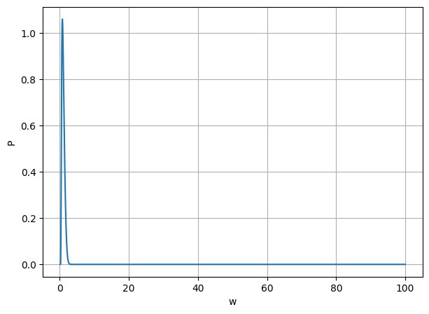
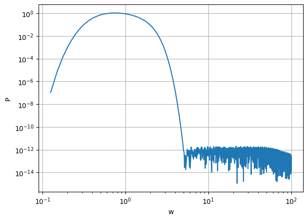
We will try to solve the equation and obtain the same result as the article. According to the authors, the solutions present power-law behavior for large values of $w$ and a cutoff behavior for small values of $w$ , in full agreement with Pareto’s observations.

Starting from the stationary equation,

\chi \left( \frac{W}{N}-w \right) P - \frac{\partial}{\partial w} \left[ \left( \frac{w^{2}}{2}A+B \right) P \right] = 0,

(206)

we choose

N=W

(207)

and

\chi=1.

(208)

We also recall that

A'=-P

(209)

and

B'=\frac{w^{2}}{2}P.

(210)

Therefore,

P = \frac{1}{1-w} \frac{\partial}{\partial w} \left[ \left( \frac{w^{2}}{2}A+B \right) P \right].

(211)

Defining

Q= \left( \frac{w^{2}}{2}A+B \right) P,

(212)

and differentiating, we obtain:

Q = \left( \frac{w^{2}}{2}A+B \right) P,

(213)

\frac{\partial Q}{\partial w} = \left( wA+\frac{w^{2}}{2}A'+B' \right)P + \left( \frac{w^{2}}{2}A+B \right)P',

(214)

Substituting the relations for $A'$ and $B'$ ,

\frac{\partial Q}{\partial w} = \left( wA-\frac{w^{2}}{2}P+\frac{w^{2}}{2}P \right)P + \left( \frac{w^{2}}{2}A+B \right)P',

(215)

and therefore,

\frac{\partial Q}{\partial w} = wAP + \left( \frac{w^{2}}{2}A+B \right)P'.

(216)

From the definition of $Q$ , the stationary equation gives:

(1-w)P = \frac{\partial Q}{\partial w}.

(217)

Equating the two expressions, we obtain:

(1-w)P = wAP + \left( \frac{w^{2}}{2}A+B \right) P'

(218)

(1-w-wA)P = \left( \frac{w^{2}}{2}A+B \right) P'

(219)

\frac{ (1-w-wA)P }{ \left( \frac{w^{2}}{2}A+B \right) } = P'.

(220)

Therefore, we have the following system of differential equations:

\frac{\partial P(w)}{\partial w} = \frac{ 1-w-wA(w) }{ \frac{w^{2}}{2}A(w)+B(w) } P(w),

(221)

\frac{\partial A(w)}{\partial w} = -P(w),

(222)

and

\frac{\partial B(w)}{\partial w} = \frac{w^{2}}{2}P(w).

(223)

Low-wealth regime

Let us consider the regime of low wealth, where

P(w)\approx0.

(224)

Then,

\frac{\partial A(w)}{\partial w}=0

(225)

and

\frac{\partial B(w)}{\partial w}=0.

(226)

Furthermore,

B \approx \int_{0}^{0} \frac{w'^{2}}{2} \frac{P(w')}{N} dw' = 0,

(227)

while

A \approx \int_{0}^{\infty} P(w')dw' = 1.

(228)

Therefore, the equation becomes:

\frac{\partial P(w)}{\partial w} = \frac{1-2w}{\frac{w^{2}}{2}} P(w).

(229)

The solution of this differential equation is

P(w) = \frac{c}{w^{4}} e^{-2/w}.

(230)

High-wealth regime

We again have

P(w)\approx0

(231)

\frac{\partial A(w)}{\partial w}=0

(232)

\frac{\partial B(w)}{\partial w}=0

(233)

B = \int_{w}^{\infty} \frac{w'^{2}}{2} \frac{P(w')}{N} dw' = B_{\infty}

(234)

A = \int_{\infty}^{\infty} P(w')dw' = 0.

(235)

Now we have:

\frac{\partial P(w)}{\partial w} = \frac{1-w}{B_{\infty}}P(w)

(236)

The solution is

P(w) = c\exp\left( \frac{(2-w)w}{2B_{\infty}} \right) = c\exp\left( \frac{(2w-w^{2})}{2B_{\infty}} \right).

(237)

Since

-(w-1)^{2}-1 = -(w^{2}-2w+1)-1 = 2w-w^{2},

(238)

then:

P(w) = c\exp\left( \frac{-(w-1)^{2}-1}{2B_{\infty}} \right)

(239)

= c\exp\left( \frac{-1}{2B_{\infty}} \right) \exp\left( \frac{-(w-1)^{2}}{2B_{\infty}} \right)

(240)

P(w) = c\exp\left( \frac{-(w-1)^{2}}{2B_{\infty}} \right).

(241)

That is, it is not exactly a power-law distribution. A numerical solution was created with the aid of DeepSeek, ChatGPT and Gemini.

import numpy as np
import matplotlib.pyplot as plt
from scipy.integrate import solve_ivp, cumulative_trapezoid
from scipy.optimize import root_scalar

# =====================================================
# PARÂMETROS
# =====================================================

chi = 2

w_start = 0.1
w_end   = 100

# =====================================================
# EVENTO DE PARADA (SINGULARIDADE)
# =====================================================

# Esta função avisa o solver quando o denominador atinge 1e-15
def limite_denominador(w, y):
    P, A, B = y
    denom = 0.5 * w * w * A + B
    return denom - 1e-15

# Comando para interromper a integração quando a função retornar 0
limite_denominador.terminal = True

# =====================================================
# SISTEMA DE EDOS (AGORA MATEMATICAMENTE PURO)
# =====================================================

def ode(w,y):

    P,A,B = y

    denom = 0.5*w*w*A + B

    # A trava artificial foi removida. O solver confia no evento.

    dP = ((chi*(1-w)-w*A)/denom)*P
    dA = -P
    dB = 0.5*w*w*P

    return [dP,dA,dB]

# =====================================================
# MÉTODO DO TIRO
# =====================================================

def shoot(P0):

    sol = solve_ivp(
        ode,
        [w_start, w_end],
        [P0, 1, 0],
        events=limite_denominador,  # <--- Evento adicionado aqui
        rtol=1e-10,
        atol=1e-12
    )

    return sol.y[1,-1]

res = root_scalar(
    shoot,
    bracket=[1e-10,2],
    method='brentq'
)

P0 = res.root

print("P inicial =", P0)

# =====================================================
# SOLUÇÃO FINAL
# =====================================================

sol = solve_ivp(
    ode,
    [w_start, w_end],
    [P0, 1, 0],
    events=limite_denominador, # <--- Evento adicionado aqui
    dense_output=True,         # Permite calcular pontos customizados depois da solução
    rtol=1e-10,
    atol=1e-12
)

# Descobrindo onde a simulação realmente parou (pode ser 100, ou antes)
w_max_real = sol.t[-1]
print(f"Integração concluída até w = {w_max_real}")

# Criando a malha exata de 4000 pontos até o limite real encontrado
w = np.linspace(w_start, w_max_real, 4000)

# Avaliando os resultados nessa nova malha usando a saída densa (sol.sol)
y_densa = sol.sol(w)

P = y_densa[0]
A = y_densa[1]
B = y_densa[2]

P inicial = 1.3656669579129148e-10
Integração concluída até w = 100.0

# @title
# =====================================================
# TESTE 1
# RESÍDUO DA EDO
# =====================================================

Q = (0.5*w**2*A+B)*P

dQ = np.gradient(Q,w)

R = chi*(1-w)*P-dQ

print()
print("========== TESTE 1 ==========")
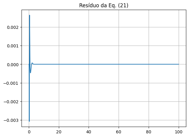
print("Resíduo máximo =",np.max(np.abs(R)))
print("Resíduo médio  =",np.mean(np.abs(R)))

# =====================================================
# TESTE 2
# RECONSTRUÇÃO DE A
# =====================================================

A_int = np.zeros_like(w)

for i in range(len(w)-1):

    A_int[i] = A_int[i] = np.trapezoid(P[i:], w[i:])

# =====================================================
# TESTE 3
# RECONSTRUÇÃO DE B
# =====================================================

B_int = cumulative_trapezoid(
    0.5*w**2*P,
    w,
    initial=0
)

print()
print("========== TESTE 2 ==========")
print("Erro máximo A =",np.max(np.abs(A-A_int)))
print("Erro máximo B =",np.max(np.abs(B-B_int)))

# =====================================================
# TESTE 4
# HIPÓTESE DO ARTIGO
# A≈1
# B≈0
# =====================================================

# Este 'mask_short_range' é específico para a região de w < 0.3
mask_short_range = w<0.3

print()
print("========== TESTE 3 ==========")

print("A médio =",np.mean(A[mask_short_range]))
print("A mínimo =",np.min(A[mask_short_range]))
print("A máximo =",np.max(A[mask_short_range]))

print()

print("B médio =",np.mean(B[mask_short_range]))
print("B máximo =",np.max(B[mask_short_range]))

# =====================================================
# TESTE 5
# EQUAÇÃO 22
# =====================================================

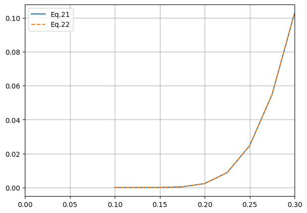
Qapprox = 0.5*w**2*P

dQapprox = np.gradient(Qapprox,w)

erro22 = np.max(np.abs(dQ[mask_short_range]-dQapprox[mask_short_range]))

print()
print("========== TESTE 4 ==========")
print("Erro aproximação Eq.22 =",erro22)

# =====================================================
# TESTE 6
# EXPOENTE LOCAL
# =====================================================

# Define uma máscara consistente para todos os gráficos log-log e cálculo de alpha
mask_for_log_plots = (P > 1e-15) & (w > 0.1)

alpha = np.gradient(
    np.log(P[mask_for_log_plots]),
    np.log(w[mask_for_log_plots])
)

# =====================================================
# GRÁFICOS
# =====================================================

plt.figure(figsize=(7,5))
plt.plot(w,P)
plt.xlabel("w")
plt.ylabel("P")
plt.grid()

plt.figure(figsize=(7,5))
plt.loglog(w[mask_for_log_plots],P[mask_for_log_plots]) # Usa a máscara consistente
plt.xlabel("w")
plt.ylabel("P")
plt.grid()

plt.figure(figsize=(7,5))
plt.plot(w,A,label="A")
plt.plot(w,A_int,"--",label="A integral")
plt.legend()
plt.grid()

plt.figure(figsize=(7,5))
plt.plot(w,B,label="B")
plt.plot(w,B_int,"--",label="B integral")
plt.legend()
plt.grid()

plt.figure(figsize=(7,5))
plt.plot(w,R)
plt.title("Resíduo da Eq. (21)")
plt.grid()

plt.figure(figsize=(7,5))
plt.plot(w[mask_short_range],dQ[mask_short_range],label="Eq.21")
plt.plot(w[mask_short_range],dQapprox[mask_short_range],'--',label="Eq.22")
plt.xlim(0,0.3)
plt.legend()
plt.grid()

#plt.figure(figsize=(7,5))
#plt.plot(w[mask_for_log_plots],alpha) # Usa a máscara consistente
#plt.axhline(-3,color='r',ls='--',label='Pareto')
#plt.xlabel("w")
#plt.ylabel(r"$d\log P/d\log w$")
#plt.legend()
#plt.grid()


# =====================================================
# DIAGNÓSTICO FINAL - EXPOENTE LOCAL
# =====================================================


========== TESTE 1 ==========
Resíduo máximo = 0.003084306495342054
Resíduo médio  = 1.3438167479948002e-05

========== TESTE 2 ==========
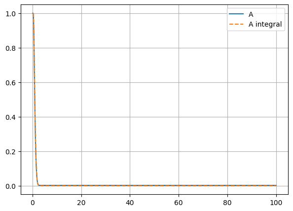
Erro máximo A = 0.002406190124915941
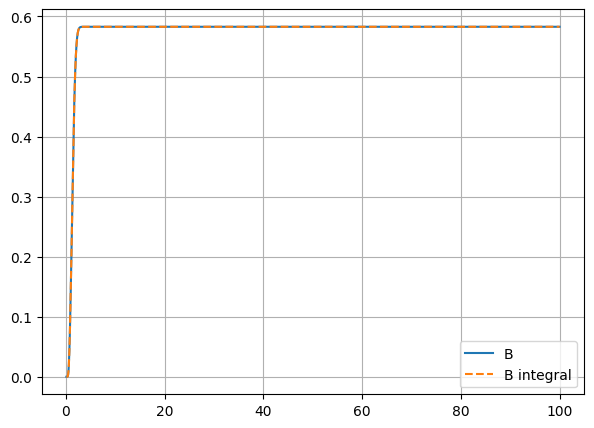
Erro máximo B = 4.542429082963692e-05

========== TESTE 3 ==========
A médio = 0.9996122233846921
A mínimo = 0.9977994902589599
A máximo = 1.0

B médio = 1.3615078697893104e-05
B máximo = 8.335080497379325e-05

========== TESTE 4 ==========
Erro aproximação Eq.22 = 9.806582728119628e-05

# =====================================================
# COMPARAÇÕES TEÓRICAS PARA w PEQUENO E w ALTO
# =====================================================

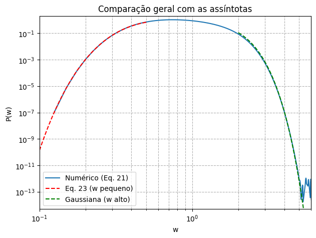
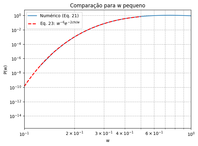
# --- 1. Ajuste da constante C para w pequeno (Eq. 23) ---
# Escolhe um ponto na região de w pequeno (ex: w ≈ 0.2)
w_ref_small = 0.2
idx_small = np.argmin(np.abs(w - w_ref_small))
C_small = P[idx_small] * (w_ref_small ** (2*(chi+1))) * np.exp(2*chi / w_ref_small)

# Gera a curva teórica para w pequeno
w_teo_small = np.linspace(w_start, 0.5, 200)  # até w=1 para ver a transição
P_teo_small = C_small * w_teo_small ** (-2*(chi+1)) * np.exp(-2*chi / w_teo_small)

# --- 2. Ajuste da constante C para w alto (Gaussiana centrada em w=1) ---
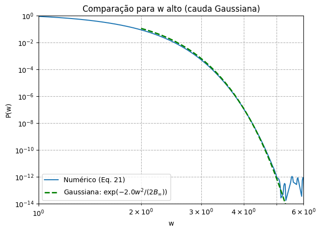
B_inf = B[-1]   # Agora SEM fator empírico!

# Escolhe um ponto na região da cauda (ex: w ≈ 4) para ajustar a constante
w_ref_high = 4.0
idx_high = np.argmin(np.abs(w - w_ref_high))
# Usando a fórmula correta: P = C * exp( chi*(2w - w^2) / (2*B_inf) )
C_high = P[idx_high] / np.exp(chi * (2*w_ref_high - w_ref_high**2) / (2 * B_inf))

# Gera a curva teórica para w alto
w_teo_high = np.linspace(2, 8, 300)
P_teo_high = C_high * np.exp(chi * (2*w_teo_high - w_teo_high**2) / (2 * B_inf))
# Forma equivalente (centrada em 1):
# P_teo_high = C_high * np.exp(-chi * (w_teo_high - 1)**2 / (2 * B_inf))

# --- 3. Gráficos de comparação ---


# (b) Comparação para w alto (log-log)
plt.figure(figsize=(7,5))
plt.loglog(w[mask_for_log_plots], P[mask_for_log_plots], label='Numérico (Eq. 21)')
plt.loglog(w_teo_high, P_teo_high, 'g--', linewidth=2, label=rf'Gaussiana: $\exp(-{chi:.1f} w^2 / (2 B_\infty))$')
plt.xlim(1, 6)
plt.ylim(1E-14, 1)
plt.xlabel('w')
plt.ylabel('P(w)')
plt.title('Comparação para w alto (cauda Gaussiana)')
plt.legend()
plt.grid(True, which='both', linestyle='--')

# (c) Comparação dupla (apenas para visualização geral)
plt.figure(figsize=(7,5))
plt.loglog(w[mask_for_log_plots], P[mask_for_log_plots], label='Numérico (Eq. 21)')
plt.loglog(w_teo_small, P_teo_small, 'r--', label='Eq. 23 (w pequeno)')
plt.loglog(w_teo_high, P_teo_high, 'g--', label='Gaussiana (w alto)')
plt.xlim(0.1, 6)
plt.ylim(5E-15, 2)
plt.xlabel('w')
plt.ylabel('P(w)')
plt.title('Comparação geral com as assíntotas')
plt.legend()
plt.grid(True, which='both', linestyle='--')
plt.show()

# (a) Comparação para w pequeno (log-log)
plt.figure(figsize=(7,5))
plt.loglog(w[mask_for_log_plots], P[mask_for_log_plots], label='Numérico (Eq. 21)')
plt.loglog(w_teo_small, P_teo_small, 'r--', linewidth=2, label=f'Eq. 23: $w^{{-{2*(chi+1)}}} e^{{-2chi/w}}$')
plt.xlim(w_start, 1.0)
plt.xlabel('w')
plt.ylabel('P(w)')
plt.title('Comparação para w pequeno')
plt.legend()
plt.grid(True, which='both', linestyle='--')

Translated with the help of GPT.