Law of Value (EBM)

Law of Value (EBM)
This model is presented in chapter 9 of the book Classical Econophysics and also as the paper: The Emergence of the Law of Value in a Dynamic Simple Commodity Economy.
Summary generated by alphavix
The paper aims to verify Marx’s claim that prices gravitate towards labor values in a simple commodity economy, where capitalist investment and profit are absent. The mathematical modeling focuses on a system of ordinary differential equations to describe the dynamics of the simple commodity economy. This approach is intended to provide an intuitive explanation of the causal features observed in the computational model, rather than definitive proofs or a precise stochastic theory. Here’s a breakdown of the key mathematical components:
Labour Equation: This equation describes how the allocation of labor to different production sectors changes over time. It’s driven by a “sectoral income error” (), which represents the difference between a sector’s actual income rate and its ideal expenditure rate needed to meet consumption demands. The rate of change of labor allocation () is proportional to this income error. In vector notation, it’s expressed as: where is the labor allocation vector, is a reaction coefficient, is the mean money velocity, is the money allocation vector, is the number of actors, is the average price vector, and is the consumption vector.
Money Equation: This equation describes how the allocation of money to different sectors changes based on the over- or under-production of commodities. It’s based on the idea that commodities in oversupply will have lower average prices, leading to a decrease in that sector’s income, and vice-versa for under-supplied commodities. The rate of change of sector income () is negatively proportional to the “production error” (), which is the difference between supply and demand for a commodity. In vector notation, it’s expressed as: where is a reaction coefficient, is a diagonal matrix of labor allocation proportions, is the labor value vector, and is the consumption vector.
Equilibrium Point and Stability: The paper shows that by setting the rates of change in both the labor and money equations to zero ( and ), a unique equilibrium point can be found. At this equilibrium, the proportion of actors in a sector equals the proportion of money received by that sector, and this proportion is equal to the ratio of labor value to consumption rate (). The paper further demonstrates the global asymptotic stability of this equilibrium point using Lyapunov’s direct method, implying that the system will always approach this equilibrium regardless of its initial conditions.
The Law of Value as an Attractor: A crucial result is Theorem 1, which states that labor values are global attractors for average market prices. This means that in equilibrium, the average price of a commodity () is proportional to the labor-time required to make it (), with a constant of proportionality () known as the Monetary Expression of Labour-time (MELT). where is the labor values vector.
Labour Commanded: The concept of “labour commanded” () is introduced as the money price of a commodity divided by the MELT. This measures how much social labor-time a commodity fetches in the market. Deviations between labor commanded and embodied labor () serve as “labour reallocation signals,” indicating over or under-valuation and guiding the adjustment of the division of labor.
In essence, the mathematical model formalizes how the dynamic interactions between labor allocation, money flows, and market prices lead to an equilibrium where prices reflect labor values and social labor is efficiently distributed, even in an economy with subjective pricing decisions.
Labor Equation
In a certain sense, this work continues the discussion started in the previous section, but now instead of an agent-based model, we have an equation-based model. We will therefore continue using the mathematical notations introduced earlier and define a few new ones.
The velocity of money is given by , where is a constant between 0 and 1.
The vector is such that each element represents the instantaneous fraction (that is, at time ) of the total money flow being received by sector .
Evidently, if we sum over all sectors we must have .
If the velocity of money is the total amount of money in circulation at a given instant , and is the fraction of that amount that sector is receiving, then clearly the total amount of money that sector is receiving is given by the product .
If the velocity of money is the total amount of money in circulation at a given instant , and is the fraction of that amount in sector , then clearly the total amount of money that sector is receiving is given by the product .
The vector is defined such that each element represents the current fraction of workers allocated in sector .
We will use the average price of the commodity to approximate the price distribution. Approximating that at each step, each agent consumes of commodity , and that its price is , then the current price cost of consumption per step per agent is .
Let us consider that agents switch sectors based on a signal indicated by prices. Each sector has an ideal expenditure rate that represents the amount of money that needs to be spent for the agents employed in this sector to satisfy their needs. This is given by the product of the individual consumption calculated previously and the current number of agents working in the sector (), that is, .
Thus, the flow, or the error in the sector’s yield rate, is given by the difference between the total money flowing into sector and the ideal consumption:
Evidently, implies that the sector has profit, that is, the sector receives more money than the agents working in it need to satisfy their consumption. On the other hand, implies a deficit, and represents the ideal equilibrium. We approximate that the switching of agents between sectors () is proportional to . For example, if there is a deficit, it means the sector does not have sufficient yield, so agents will leave the sector in search of another sector that is profitable and capable of absorbing them. In other words, , where is a positive constant that regulates the intensity of sector switching.
This is the labor equation: it defines how the allocation of labor across different production sectors varies according to the yield received by the sector from the sale of commodities. We can write it in a more complete form:
Recalling that the consumption vector is given by , and that we previously defined a price vector , then .
Thus, the labor equation for the entire economy can be written in vector notation as:
Now, since an agent in sector produces units of the commodity at each step (it is produced after steps), the total production in the sector is given by .
If we define the average price of commodity as the result of dividing the sector’s income (as we saw earlier, given by ) by the total quantity of commodities produced, that is, the money that entered the sector from the sale of commodities divided by the quantity of commodities produced, then the average price is:
Money Equation
We now want to understand how the change in income depends on the distribution of labor. Certainly, a sector’s income depends on the quantity of commodities produced. Since no one consumes more than they need, the maximum consumption corresponds to the “social demand” for each commodity .
As each agent consumes per step (meaning they consume one unit of the commodity every steps), the social demand is given by . Similarly, each agent employed in sector produces , and since the number of agents in the sector is , the total amount of commodity produced in the sector is .
Thus, analogous to what we did previously, the flow, or the production error given by the difference between the quantity of commodity produced and consumed, is given by:
Evidently, represents overproduction, and implies that not enough is being produced, while denotes equilibrium. If we assume that when there is overproduction (underproduction) the price falls (rises), then the change in sector income is proportional, but inversely, to , that is, , where is a positive constant that adjusts the intensity with which the income distribution reacts to the production error.
This equation is known as the money equation because it defines how the allocation of money across different sectors varies according to overproduction or underproduction of commodities. It can be written in a more complete form as:
If we define a matrix where the only nonzero elements are the diagonal elements , and using the production vector as a column vector, we can write the money equation for the entire economy as:
Since the consumption vector is , we will now investigate how the equilibrium of this system, formed by the labor and money equations, is achieved.
Equilibrium
Bringing together the previous results, we have that a simple commodity system is described by the following system of coupled differential equations (the labor equation and the money equation for the entire economy):
Where:
And with the following constraints:
And:
() is the total amount of money (population) in the system.
is the fraction of workers producing commodity at a given moment in time. is then the number of workers in sector , and is the vector formed by the elements . Meanwhile, is a matrix where the only nonzero elements are the diagonal elements , which are the elements .
is the fraction of money exchanged per unit of time, so is the velocity of money.
is the fraction of received by the sector producing commodity at a given time, and is the vector formed by the elements .
() is the time required for a commodity to be produced (consumed). () is the vector formed by the elements ().
() is a constant that regulates the intensity with which workers (income) migrate between sectors.
is the average price of commodity , and is the vector formed by the elements .
In summary, this system works according to the following scheme: a certain division of labor results in over or underproduction of commodities, which activates a price correction mechanism based on supply and demand. This causes a change in sector income, which consequently leads agents to switch sectors, resulting in a new division of labor.
This system has a single equilibrium point given by:
To facilitate understanding, let us first revisit the equations for a single sector :
Considering the equilibrium situation, that is, when there are no more variations ():
Or simply:
From the second equation, we directly obtain:
Substituting into the first equation, and also replacing the definition of the average price, we have:
Substituting again (a term that reappeared because of ):
And since , then:
That is, when the system is in equilibrium, the proportion of agents employed in each sector is equal to the proportion of money each sector receives, which is proportional to . This makes sense because all agents in this model require the same income to satisfy their needs. We had already shown that the efficient division of labor occurs when , so a result we obtain without much effort is that, at equilibrium, the division of labor tends to maximum efficiency.
Furthermore, this equilibrium point is asymptotically stable, that is, regardless of the initial conditions, the system always evolves toward the equilibrium point. To prove this, we first need to a) linearize the system and b) shift the equilibrium point to the origin, then we can apply Lyapunov’s direct method.
The equations are:
We need to linearize the first term. First, since , it follows that , because the variation in each element must be ‘cancelled’ by an equivalent variation of opposite sign in another (or other) elements so that the sum remains constant. Thus:
Where we use the fact that .
Revisiting our equation then:
That is:
Now, with a simple change of variables and , we shift the equilibrium point to the origin. With this change, for the labor equation, we have:
Ou em notação vetorial:
And for the money equation:
Or in vector notation:
We then have:
Or:
Analogously to , is the matrix where only the diagonal elements are nonzero. Since the equilibrium is now at the origin, the terms and represent an error in production and income in sector .
To formalize this, we define a function , meaning that assigns a real number to each vector of variables . This function allows us to assign a scalar value to each configuration of the system. More explicitly:
We thus have a scalar measure of the error for each possible state of our system. Obviously, if we are at the origin , then , and if we are away from the origin, then , since and are real numbers greater than or equal to zero. All terms are necessarily non-negative, and the choice of this specific form for is to simplify later calculations.
What we want is for to be a Lyapunov function. For this to be possible, must first satisfy at the origin and in the neighborhood of the origin. As discussed, both cases are satisfied with this definition of . The last requirement is that . Taking the derivative:
Since the derivative of a sum is the sum of the derivatives, substituting and :
Or simply:
Evidently, , as we wanted. Moreover, occurs only for ; in all other cases, we have . That is, the scalar error given by always decreases over time until equilibrium is reached, where the error is zero and then stabilizes. in the neighborhood of the equilibrium point is what defines a point as asymptotically stable. In this case, since the Lyapunov function is valid for all of and not just near the equilibrium point, we can say that the point is globally asymptotically stable.
Finally, we can reach the result that interests us most: the law of value. Labor values are attractors for the average prices. That is:
Where . Since denotes how many units of commodity are produced per unit of time, denotes how many units of time are required to produce commodity . Returning to the definition of the average price and using the equilibrium point (), we have:
Where evidently we then have , representing the monetary value of one unit of labor-time. As the system tends toward equilibrium, the prices tend toward .
It is interesting to note that the numerator of is the same as that calculated for the simulation: the velocity of money. But the denominator is different. We must remember that the denominator is the labor expended and exchanged in the market over a given time interval. If our time interval is one unit, and we have agents in a system where all agents are always necessarily producing, then in one unit of time, units of labor-time are incorporated into the commodities.
Since we are analyzing only the goods being exchanged in the market, we can see on average, units of labor-time are exchanged per unit of time. We can also note that, in a way, when agents switch sectors seeking to maximize their income, they always try to work in a sector where the commodity they produce will be better sold.
Conclusion
The quantitative part of Marxist value theory tells us that prices are related to the socially necessary labor time required to produce a commodity, and deviations of prices from values are signals of social errors that serve to redistribute labor. To analyze this more closely, let us define the concept of labour commanded: .
This quantity represents how much socially necessary labor time, on average, a commodity “contains” when it is exchanged in the market. Recall that the MELT, or “Monetary Expression of Labor Time,” has units of money per unit of labor-time. Since the price is in money, has units of labor-time. If , this means the commodity has been traded at a depreciated price; obviously, if , then the commodity is overvalued. Evidently, all these quantities are objective and independent of any individual subjectivity about the utility of the commodity, and at equilibrium .
Manipulating the necessary labor, it can be rewritten as:
That is, . Substituting into the linearized version of the labor equation, we have:
Or simply:
Looking at the term in parentheses, if , then the subtraction is positive and the commodity is overvalued, signaling the need to expand the sector and increase its production. Evidently, signals the opposite. It is worth noting that the equilibrium we are working with is a statistical equilibrium, meaning we are discussing an ‘average’ relationship between value and price. Even at equilibrium, an individual transaction can occur at different prices. The law of value, as presented, states that at equilibrium, the average price of commodities is proportional to their labor values.
It is important to note that this model does not exhaust the possibilities for investigating the topic. There are models that explore, for example, complex production systems where one commodity is required to produce another (Krause), but I believe that for a first contact, the content presented here already fulfills its purpose.
If we define a coefficient , which indicates that 1 hour of labor in the production of commodity is equivalent to hours of labor in commodity , we can then write:
First of all, we can note that gives us the amount of money that one unit of labor-time in the production of commodity is measured in money. So, when we divide this amount for commodity by the corresponding amount for commodity , we obtain the “price” of one unit of labor-time in the production of commodity expressed in units of labor-time for the production of commodity .
In other words, this ratio “indicates that 1 hour of labor in the production of commodity is equivalent to hours of labor in commodity .” For example, if commodity has 2 units of money per unit of labor-time and commodity has 4, then , meaning that for each time interval in which commodity is equivalent to 1 unit of money, this time corresponds to 0.5 units of money for commodity .
We have already obtained the result that at equilibrium , so evidently at equilibrium , and consequently . In other words, the statement that values are attractors for prices at equilibrium is equivalent to the statement that homogeneous coefficients are attractors for heterogeneous coefficients at equilibrium.
The law of value is a dynamic theory of labor allocation based on the tendency of heterogeneous labor to be homogenized through commodity exchange. Evidently, this is an idealized scenario that allows us to understand some fundamental concepts for analyzing capitalism and is far from exhausting the subject.
In conclusion, the law of value is a phenomenon that emerges from the dynamic interaction of private commodity producers. In the model presented: values are global attractors for prices, prices in turn act as signals of errors that work to allocate the social division of available labor more efficiently across sectors, and the tendency of prices to approach value is the monetary expression of the tendency to allocate social labor efficiently. The MELT is an interesting constant because it summarizes a non-obvious relationship between a production phenomenon (production time) and a market phenomenon (prices). With the definition of labour commanded, we can have an indirect signal of whether the labor in the production of that commodity is socially necessary or not.
Perhaps most interestingly, the law of value operates “behind the scenes”; it emerges naturally from the system dynamics and does not need to be imposed directly at any point. It is also worth noting that the system’s equilibrium is statistical, meaning we look at the average price of a commodity, which can individually be exchanged at different prices even when the system reaches equilibrium. Moreover, the law of value can only emerge in an economic system that contains a feedback cycle between production, consumption, exchange, and the reallocation of labor resources.
import numpy as np
from scipy.integrate import solve_ivp
import matplotlib.pyplot as plt
# System parameters
psi = 0.1
gamma = 0.01
M = 1.0
omega = 0.01
N = 1.0
l = np.array([1,2]) # l1, l2
c = np.array([3, 3]) # c1, c2
# Initial conditions
a0 = np.array([1/3, 2/3]) # a1(0), a2(0)
b0 = np.array([0.5, 0.5]) # b1(0), b2(0)
y0 = np.concatenate((a0, b0)) # Initial state vector
# Model
def model(t, y):
a1, a2, b1, b2 = y
S = (l[0]*b1)/(c[0]*a1) + (l[1]*b2)/(c[1]*a2)
da1dt = psi*gamma*M*(b1 - a1*S)
da2dt = psi*gamma*M*(b2 - a2*S)
db1dt = -omega*N*(a1/l[0] - 1/c[0])
db2dt = -omega*N*(a2/l[1] - 1/c[1])
return [da1dt, da2dt, db1dt, db2dt]
#N(M) is just a quantity of workers (money). The total quantity of workers (money) at any given moment is not necessarily constant. In equilibrium, only Σaj=1 is guaranteed, since in equilibrium aj=lj/cj and we define the parameters cj and lk such that Σlj/cj=1. Outside of equilibrium, there is no guarantee that Σaj=bj=1.
#This is an additional and special constraint. All other constraints depend on the parameters, but this constraint is a set of additional equations beyond the system of differential equations.
#To ensure this constraint, we will apply normalization at each step.
#Note: It is possible to improve accuracy, but I believe the result is sufficient.
# Normalization
def normalize(y):
y = y.copy()
a_total = y[0] + y[1]
b_total = y[2] + y[3]
y[0] /= a_total
y[1] /= a_total
y[2] /= b_total
y[3] /= b_total
return y
#I think that another option is to use the restriction to reduce the dimensions of the system in two equations, writing the last one as the one minus the sum of the others. So, if we've got L commodity, we don't have 2L equations, but 2L-2. I guess this is the most elegant solution, and I thought of it late, so I'll just put this note here.
# Initial state
y = y0
t0, tf, dt = 0, 10000, 0.01
t_values = [t0]
y_values = [y]
t = t0
while t < tf:
# Integrate a small step
sol = solve_ivp(model, [t, t+dt], y, method='RK45')
y_new = sol.y[:, -1]
# Normalize before storing and using as initial condition
y_new = normalize(y_new)
# Store and update for the next step
y_values.append(y_new)
y = y_new
t += dt
t_values.append(t)
# Convert to array
y_values = np.array(y_values)
t_values = np.array(t_values)
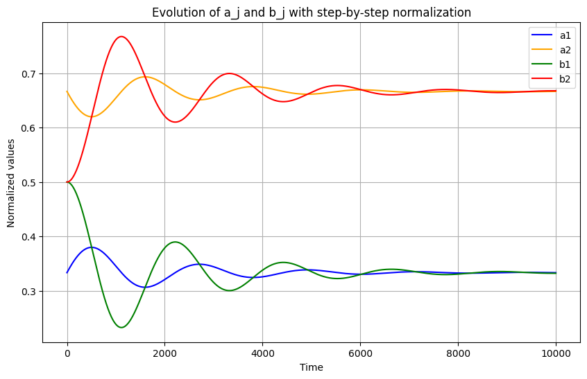
# Plot
plt.figure(figsize=(10,6))
plt.plot(t_values, y_values[:,0], label='a1', color='blue')
plt.plot(t_values, y_values[:,1], label='a2', color='orange')
plt.plot(t_values, y_values[:,2], label='b1', color='green')
plt.plot(t_values, y_values[:,3], label='b2', color='red')
plt.xlabel('Time')
plt.ylabel('Normalized values')
plt.title('Evolution of a_j and b_j with step-by-step normalization')
plt.legend()
plt.grid(True)
plt.show()
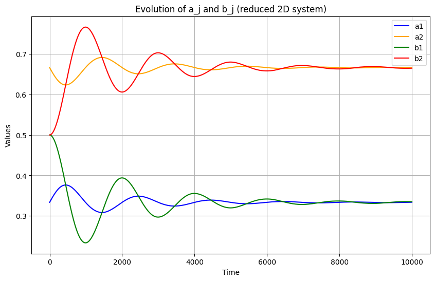
#I'm kidding, I have trouble knowing when to stop, so here is the reduced system with 2L-2 equations for L=2. Did you know that I didn't sleep last night thinking about this? And it still bothers me that my result is not exact in the computational version of this model.

import numpy as np
from scipy.integrate import solve_ivp
import matplotlib.pyplot as plt


# System parameters
psi = 0.1
gamma = 0.01
M = 1.0
omega = 0.01
N = 1.0
l = np.array([1,2])  # l1, l2
c = np.array([3, 3])   # c1, c2

# Initial conditions
a0 = np.array([1/3])  # a1(0), a2(0)
b0 = np.array([0.5])  # b1(0), b2(0)
y0 = np.concatenate((a0, b0))  # Initial state vector


# Reduced model using normalization a2 = 1-a1, b2 = 1-b1
def model_reduced(t, y):
    a1, b1 = y
    a2 = 1 - a1
    b2 = 1 - b1

    # S term
    S = (l[0]*b1)/(c[0]*a1) + (l[1]*b2)/(c[1]*a2)

    # Derivatives for independent variables
    da1dt = psi*gamma*M*(b1 - a1*S)
    db1dt = -omega*N*(a1/l[0] - 1/c[0])

    return [da1dt, db1dt]

# Integration
t_eval = np.linspace(0, 10000, 1000)
sol = solve_ivp(model_reduced, [0, 10000], y0, t_eval=t_eval, method='RK45')

# Recover full variables
a1 = sol.y[0]
a2 = 1 - a1
b1 = sol.y[1]
b2 = 1 - b1

# Plot
plt.figure(figsize=(10,6))
plt.plot(sol.t, a1, label='a1', color='blue')
plt.plot(sol.t, a2, label='a2', color='orange')
plt.plot(sol.t, b1, label='b1', color='green')
plt.plot(sol.t, b2, label='b2', color='red')
plt.xlabel('Time')
plt.ylabel('Values')
plt.title('Evolution of a_j and b_j (reduced 2D system)')
plt.legend()
plt.grid(True)
plt.show()
- Wright, I. (2008). The Emergence of the Law of Value in a Dynamic Simple Commodity Economy. Review of Political Economy, 20(3), 367–391. 10.1080/09538250701661889