Kinetic model with a marginalist approach

This is an automatically generated summary by Gemini: This Jupyter Notebook analyzes critically the kinetic models of monetary exchange from the perspective of econophysics, evaluating the attempts to establish their microeconomic foundations through the marginalist microeconomic approach based on Cobb-Douglas utility functions and budget constraints optimized by Lagrange multipliers. The text analytically demonstrates that, although these models attempt to incorporate elements of the productive sphere and competitive equilibrium, the exchange dynamics ultimately reduce to pure stochastic processes of wealth redistribution (guided by random sharing coefficients) where assumptions such as agent homogeneity and perfect equilibrium hollow out the real economic content and mask structural contradictions of capitalism. Furthermore, the work extends the discussion to generalized models with exogenous interest rates and growing markets, concluding that the Marxist conceptual framework can offer greater methodological consistency for interpreting such systems than the traditional marginalist approach.

This is a different article that seeks to rely in part on marginalist theory as presented in the paper “Microeconomics of the ideal gas like market models”. Let us assume:

Agent $i$ produces only $Q_{i}$ units of commodity $i$ , and their money at time $t$ is given by $m_{i}(t)$ .
- Notice that, although this is a model that attempts to provide a microeconomic justification within marginalism, it assumes a condition of equality in the market among all agents as producers and consumers. Such equality does not exist, not only materially but also legally, since private ownership of the means of production assigns different roles to each agent in the production process.
We want to understand how the money held by agent $m_{i}(t)$ varies over time $t$ .
Considering an exchange between two agents $i$ and $j$ , we define a utility function given by $U_{i}(x_{i}, x_{j}, m_{i}) = x_{i}^{\alpha_{i}} x_{j}^{\alpha_{j}} m_{i}^{\alpha_{m}},$ where $x_{i}$ and $x_{j}$ denote the consumption of commodities $i$ and $j$ by the agent in question.
- A utility function measures the consumer’s preferences and satisfaction with different goods or services. It is important to stress that there is a certain arbitrariness in choosing such a specific functional form. The chosen function is called Cobb–Douglas and is popular in marginalist literature.
For convenience, we denote $m_{i}(t+1)=m_{i}$ and $m_{i}(t)=M_{i}$ .
For simplicity, we also assume that $\alpha_{i}+\alpha_{j}+\alpha_{m}=1$ .

Denoting the price of commodity $i$ by $p_{i}$ , we then define a budget constraint for agent $i$ as:

p_{i}x_{i}+p_{j}x_{j}+m_{i}\leq M_{i}+p_{i}Q_{i}

(1)

In other words, the amount that agent $i$ can spend by consuming quantities $x_{i}$ and $x_{j}$ of the two commodities, together with the money they retain after the exchange, cannot exceed the money they possessed in the previous time step plus the revenue obtained from selling the commodity they produce. Indeed, since $x_{i}$ represents consumption, then $p_{i}x_{i}+p_{j}x_{j}=\Delta m_{i}$ corresponds to the monetary flow spent on consumption. Likewise, if we denote $p_{i}Q_{i}=\Delta M_{i}$ as the monetary flow earned from production, we can rewrite the budget constraint as

\Delta m_{i}+m_{i}\leq M_{i}+\Delta M_{i}.

(2)

In fact, for a conservative system we necessarily have

\Delta m_{i}+m_{i}=M_{i}+\Delta M_{i}.

(3)

The idea is that agents seek to maximize their utility functions. Given, then, the utility function and the constraints:

\begin{aligned} U_{i}(x_{i},x_{j},m_{i}) &= x_{i}^{\alpha_{i}}x_{j}^{\alpha_{j}}m_{i}^{\alpha_{m}},\ p_{i}x_{i}+p_{j}x_{j}+m_{i}-M_{i}-p_{i}Q_{i} &= 0. \end{aligned}

To optimize a function subject to a constraint, we can use the trick of the Lagrange multiplier. First, we construct the Lagrangian.

L= U_{i}\left(x_{i},x_{j},m_{i}\right)+\lambda g = x^{\alpha_{i}}_{i}x^{\alpha_{j}}_{j}m^{\alpha_{m}}_{i}+\lambda p_{i}x_{i}+\lambda p_{j}x_{j}-\lambda M_{i}+\lambda m_{i}

(4)

We may note that the condition $g=0$ is satisfied only for a specific set of values of the variables, which, in practice, correspond to the only admissible states of the system. On this constraint surface, we have $L=U_{i}+\lambda g=U_{i}$ , since $g=0$ .

We now differentiate the Lagrangian with respect to the variables. Recall that $p_{i}x_{i}+p_{j}x_{j}+m_{i}\leq M_{i}+p_{i}Q_{i}$ , where all the variables appear on the left-hand side of the inequality. Thus, we are deciding the best transaction to make at time $t+1$ , given a previous state of $m_{i}\left(t\right)$ and $Q_{i}\left(t\right)$ at time $t$ .

0=\frac{\partial L}{\partial x_{i}}= \alpha_{i}x^{\alpha_{i}-1}_{i}x^{\alpha_{j}}_{j}m^{\alpha_{m}}_{i}+\lambda p_{i}

(5)

0=\frac{\partial L}{\partial x_{j}}= \alpha_{j}x^{\alpha_{i}}_{i}x^{\alpha_{j}-1}_{j}m^{\alpha_{m}}_{i}+\lambda p_{j}

(6)

0=\frac{\partial L}{\partial m_{i}}= \alpha_{m}x^{\alpha_{i}}_{i}x^{\alpha_{j}}_{j}m^{\alpha_{m}-1}_{i}+\lambda

(7)

0=\frac{\partial L}{\partial\lambda}= p_{i}x_{i}+p_{j}x_{j}+m_{i}-M_{i}-p_{i}Q_{i}

(8)

Since we seek the prices at which the commodities should be exchanged at this optimum point:

p_{i}= -\frac{\alpha_{i}x^{\alpha_{i}-1}_{i}x^{\alpha_{j}}_{j}m^{\alpha_{m}}_{i}}{\lambda}

(9)

p_{j}= -\frac{\alpha_{j}x^{\alpha_{i}}_{i}x^{\alpha_{j}-1}_{j}m^{\alpha_{m}}_{i}}{\lambda}

(10)

\lambda= -\alpha_{m}x^{\alpha_{i}}_{i}x^{\alpha_{j}}_{j}m^{\alpha_{m}-1}_{i}

(11)

Substituting $\lambda$ into $p_{i}$ :

p_{i}=\frac{\alpha_{i}x^{\alpha_{i}-1}_{i}x^{\alpha_{j}}_{j}m^{\alpha_{m}}_{i}}{\alpha_{m}x^{\alpha_{i}}_{i}x^{\alpha_{j}}_{j}m^{\alpha_{m}-1}_{i}} =\frac{\alpha_{i}}{\alpha_{m}}\frac{m^{\alpha_{m}}_{i}}{m^{\alpha_{m}-1}_{i}}\frac{x^{\alpha_{i}-1}_{i}}{x^{\alpha_{i}}_{i}} =\frac{\alpha_{i}}{\alpha_{m}}\frac{m_{i}}{x_{i}}

(12)

Similarly, for $p_{j}$ :

p_{j}=\frac{\alpha_{j}x^{\alpha_{i}}_{i}x^{\alpha_{j}-1}_{j}m^{\alpha_{m}}_{i}}{\alpha_{m}x^{\alpha_{i}}_{i}x^{\alpha_{j}}_{j}m^{\alpha_{m}-1}_{i}} =\frac{\alpha_{j}}{\alpha_{m}}\frac{m_{i}}{x_{j}}

(13)

To actually solve the problem, we need to determine the values of the variables at the optimized equilibrium $\left(x^{*}_{i},x^{*}_{j},m^{*}_{i}\right)$ . We can rewrite the previous expressions as

p_{j}x^{*}_{j}=\frac{\alpha_{j}}{\alpha_{m}}m^{*}_{i},\qquad x^{*}_{i}p_{i}=\frac{\alpha_{i}}{\alpha_{m}}m^{*}_{i}

(14)

And from the last equation, $\partial L/\partial\lambda$ , we have

\frac{\alpha_{j}}{\alpha_{m}}m^{*}_{i}+\frac{\alpha_{i}}{\alpha_{m}}m^{*}_{i}+m^{*}_{i}-M_{i}-p_{i}Q_{i}=0

(15)

\left(\frac{\alpha_{j}}{\alpha_{m}}+\frac{\alpha_{i}}{\alpha_{m}}+1\right)m^{*}_{i} =M_{i}+p_{i}Q_{i}

(16)

m^{*}_{i} =\alpha_{m}\frac{M_{i}+p_{i}Q_{i}}{\left(\alpha_{j}+\alpha_{i}+\alpha_{m}\right)} =\alpha_{m}\left(M_{i}+p_{i}Q_{i}\right)

(17)

where we have used the fact that $\alpha_{j}+\alpha_{i}+\alpha_{m}=1$ .

Combining the previous results, we can eliminate $m^{*}_{i}$ from $p_{k}$ and write:

m^{*}_{i}=\alpha_{m}\left(M_{i}+p_{i}Q_{i}\right)

(18)

x^{*}_{j}=\alpha_{j}\frac{\left(M_{i}+p_{i}Q_{i}\right)}{p_{j}}

(19)

x^{*}_{i}=\alpha_{i}\frac{\left(M_{i}+p_{i}Q_{i}\right)}{p_{i}}

(20)

And if we impose equilibrium between demand and consumption—notice that we are imposing a perfect equilibrium, which is highly unrealistic. At the same time that the model seeks to simulate capitalism in a more realistic way, the resources required for commodity production are assumed to be infinite (in every respect, the agent does not need money to produce) and free of charge—in the transaction between agents $i$ and $j$ , then for agent $j$ we have $U_{j}\left(y_{i},y_{j},m_{j}\right)$ . Notice that we now have four consumption variables, $\left\{x_{i},x_{j},y_{i},y_{j}\right\}$ , in order to describe the consumption of both agents for both commodities. However, the coefficients—that is, the preferences for the commodities—are the same, $\left\{\alpha_{i},\alpha_{j},\alpha_{m}\right\}$ , for both agents involved. This homogeneity of preferences is a restriction that the author does not make explicit. Then $x_{k}+y_{k}=Q_{k}$ . For agent $j$ , we analogously obtain

m^{*}_{j}=\alpha_{m}\left(M_{j}+p_{j}Q_{j}\right)

(21)

y^{*}_{j}=\alpha_{j}\frac{\left(M_{j}+p_{j}Q_{j}\right)}{p_{j}}

(22)

y^{*}_{i}=\alpha_{i}\frac{\left(M_{j}+p_{j}Q_{j}\right)}{p_{i}}

(23)

Furthermore, considering that the total amount of money remains constant, $m_{i}+m_{j}=M_{i}+M_{j}$ . In the paper, this is presented later as if it were deduced from the optimal prices obtained, but we actually need to assume this condition in order to derive those optimal prices. At least, I could not find another way to obtain the same optimal prices. That is,

M_{i}+M_{j}=m^{*}_{i}+m^{*}_{j}=\alpha_{m}\left(M_{i}+M_{j}+p_{i}Q_{i}+p_{j}Q_{j}\right)

(24)

Alternatively, if we define $M_{i}+p_{i}Q_{i}=R_{i}$ as the wealth (the sum of the money and the value of the commodities owned) of agent $i$ at time $t$ , then

m^{*}_{i}=\alpha_{m}R_{i}

(25)

x^{*}_{j}=\alpha_{j}\frac{R_{i}}{p_{j}}

(26)

x^{*}_{i}=\alpha_{i}\frac{R_{i}}{p_{i}}

(27)

m^{*}_{j}=\alpha_{m}R_{j}

(28)

y^{*}_{j}=\alpha_{j}\frac{R_{j}}{p_{j}}

(29)

y^{*}_{i}=\alpha_{i}\frac{R_{j}}{p_{i}}

(30)

M_{i}+M_{j}=\alpha_{m}\left(R_{i}+R_{j}\right)

(31)

Summing, we obtain

x^{*}_{i}+y^{*}_{i}=\alpha_{i}\frac{R_{i}}{p_{i}}+\alpha_{i}\frac{R_{j}}{p_{i}}

(32)

Q_{i}p_{i}=\alpha_{i}\left(R_{i}+R_{j}\right)

(33)

p_{i}=\frac{\alpha_{i}}{\alpha_{m}}\frac{M_{i}+M_{j}}{Q_{i}}

(34)

Similarly, for commodity $j$ we have

p_{j}=\frac{\alpha_{j}}{\alpha_{m}}\frac{M_{i}+M_{j}}{Q_{j}}.

(35)

Before proceeding, let us assume that $\alpha_{i}$ can vary randomly over time while $\alpha_{m}$ remains constant. Then we have

\alpha_{j}=1-\alpha_{m}-\alpha_{i}.

(36)

Furthermore, let us define $\alpha_{m}=\lambda$ and

\epsilon=\frac{\alpha_{i}}{\alpha_{i}+\alpha_{j}}.

(37)

As we shall see later, $\lambda\in\left[0,1\right]$ is the propensity to save, while $\epsilon\in\left[0,1\right]$ is the fraction of the total money of both agents that will be transferred to agent $i$ . That is, if $\lambda=0$ and $\epsilon=1$ , then all of agent $j$ ’s money is transferred to agent $i$ ; if $\epsilon=0$ , we obtain the opposite result. We can write the money transfer equations between the agents as

m_{i}\left(t+1\right) =\lambda m_{i}\left(t\right) +\left(1-\lambda\right)\left[m_{i}\left(t\right)+m_{j}\left(t\right)\right]\epsilon

(38)

m_{j}\left(t+1\right) =\lambda m_{j}\left(t\right) +\left(1-\lambda\right)\left[m_{i}\left(t\right)+m_{j}\left(t\right)\right]\left(1-\epsilon\right)

(39)

Let us prove this. Using the equations for $m^{*}_{i}$ and $p_{i}$ , we obtain for agent $i$

m^{*}_{i} =\alpha_{m}\left(M_{i}+p_{i}Q_{i}\right)

(40)

m_{i}\left(t+1\right) =\alpha_{m}m_{i}\left(t\right) +\alpha_{m}\left(\frac{\alpha_{i}}{\alpha_{m}}\frac{m_{i}\left(t\right)+m_{j}\left(t\right)}{Q_{i}}\right)Q_{i}

(41)

=\alpha_{m}m_{i}\left(t\right) +\alpha_{i}\left[m_{i}\left(t\right)+m_{j}\left(t\right)\right]

(42)

where we have defined $\alpha_{m}=\lambda$ . Since $1-\alpha_{m}=\alpha_{i}+\alpha_{j}$ , we have

\frac{1-\alpha_{m}}{\alpha_{i}+\alpha_{j}}=1.

(43)

Thus,

m_{i}\left(t+1\right) =\alpha_{m}m_{i}\left(t\right) +\frac{\alpha_{i}}{\alpha_{i}+\alpha_{j}} \left(1-\alpha_{m}\right) \left[m_{i}\left(t\right)+m_{j}\left(t\right)\right].

(44)

And since we have defined

\epsilon=\frac{\alpha_{i}}{\alpha_{i}+\alpha_{j}},

(45)

we obtain the equation for $m_{i}\left(t+1\right)$ . An analogous derivation can be carried out for $m_{j}\left(t+1\right)$ .

More directly, this equation shows that the model essentially consists of two mechanisms: (1) a fixed parameter $\alpha_{m}$ that determines the agents’ propensity to save; and (2) a random fraction $\alpha_{i}\in[0,1-\alpha_{m}]$ of the total wealth involved in the interaction, which determines how much of the combined wealth is appropriated by agent $i$ . In this sense, the effective dynamics of the exchange reduce to a stochastic process of monetary redistribution. The original marginalist interpretation loses much of its substantive content, since the exponents of the utility function no longer represent economically determined preferences, but instead act merely as random sharing coefficients.

Observe that, although the model starts from Cobb-Douglas utility functions, the effective dynamics of the exchanges end up being governed by a single random variable, $\epsilon$ , which determines how the monetary redistribution between the agents occurs in each transaction. Since the exponents satisfy $\alpha_{1}+\alpha_{2}+\alpha_{m}=1$ , and $\alpha_{m}=\lambda$ is taken to be constant, it follows that $\alpha_{1}+\alpha_{2}=c=1-\lambda$ . Therefore, only one independent degree of freedom remains. We may then parametrize the exponent as

\alpha_{1}=\epsilon c.

(46)

Thus, if $\alpha_{1}$ is uniformly distributed over the interval $\alpha_{1}\in[0,1-\lambda]$ , then $\epsilon$ is also uniformly distributed over $[0,1]$ , differing only by a rescaling factor. Consequently, the resulting dynamics coincide with the classical kinetic exchange models of money.

Therefore, this procedure not only reproduces the classical random exchange models, but also suggests that the marginalist microfoundation loses part of its original economic content. The exponents of the utility function, which in principle would represent the agents’ preferences, instead act merely as random coefficients governing the monetary sharing rule. Furthermore, because the model imposes perfect equilibrium between supply and demand at every interaction, exchange no longer reflects the decentralized process characteristic of real capitalist economies, but instead resembles a purely stochastic dynamics of wealth redistribution.

Likewise, the assumption that every agent acts simultaneously as both producer and consumer under symmetric conditions also makes it difficult to provide a faithful representation of the capitalist mode of production. Such a limitation is often tolerated in simpler models that completely abstract from the sphere of production. In the present case, however, the model explicitly seeks to incorporate production into its microeconomic foundation. Thus, by introducing the productive sphere while preserving a symmetric structure among the agents, it ultimately strips away fundamental elements of capitalist dynamics.

Furthermore, it is worth emphasizing that, once the classical econophysics model is recovered, we obtain essentially the same results that are already well established in the literature. At this point, it is interesting to note that these results often differ from the conclusions typically expected by proponents of the marginalist approach to economics, particularly in its liberal interpretations.

In particular, the model does not suggest that the free market necessarily leads to a socially optimal distribution of wealth. Likewise, the resulting inequality cannot be attributed to differences in ability, productivity, or individual merit, since the agents are assumed to be homogeneous in their fundamental characteristics.

Thus, although the discussion is formulated in terms of marginalist microeconomic foundations and assumptions of competitive equilibrium, the results obtained are not consistent with the traditional normative interpretations commonly associated with the free market, especially those that attribute economic inequality to individual differences in competence or efficiency.

When $\lambda=0$ , we have the traditional exchange kinetic model:

m_{i}\left(t+1\right) =\left(m_{i}\left(t\right)+m_{j}\left(t\right)\right)\epsilon

(47)

m_{j}\left(t+1\right) =\left(m_{i}\left(t\right)+m_{j}\left(t\right)\right)\left(1-\epsilon\right)

(48)

Generalized Model¶

Remark: In fact, this is not merely a “generalization,” but rather a different class of models. Unlike the previous model, which describes the exchange of wealth between agents, this one instead models, in a certain sense, the wealth growth of an individual agent. The market, contrary to what is stated, is more than just an “intermediary”; it acts both as a source and as a sink of money. Indeed, there is as much motivation for saying that the agents exchange wealth with one another as there is for claiming that they never exchange wealth at all, since the evolution of each agent’s wealth ultimately becomes, to a large extent, independent of the others. In the end, the evolution of an agent’s wealth depends only on that agent’s own parameters.

I chose to restrict the distribution of one parameter, $\alpha_{i}\left(t\right)$ , in order to preserve the conservation of money in the system and make the market effectively function as an intermediary between the agents. In the original argument, however, this restriction can be relaxed, making the evolution of each agent largely independent. This represents a change of model that is not made explicit in the article. In particular, in the model used for comparison—where $\alpha_{i}\left(t\right)$ is replaced by a white noise term $\xi_{i}\left(t\right)$ , and which the article seeks to approximate— is not, in fact, an interacting-agent model. In practice, it is simply a model describing the evolution of the wealth of an individual agent.

Up to this point, we have worked with a pricing mechanism that operates only locally, between two agents, in order to balance supply and demand within their bilateral interaction. We now seek to generalize this framework so that prices are determined globally.

In this formulation, the market is described as a black box in which agents interact only indirectly through the market itself. The proposed dynamics are as follows:

Each agent seeks to maximize the utility function

U\left(f,c\right)=f^{\lambda}c^{\left(1-\lambda\right)},

(49)

where:

$f\rightarrow$ is the amount of money available for future consumption, obtained from the money saved today for that purpose after earning the market rate of return $r$ .
$c\rightarrow$ is the amount of money allocated to present consumption.

In other words, the agent must decide how to allocate their financial resources between present consumption and investment for future consumption, taking into account a market return factor $r$ . The budget constraint is

m\left(t\right)=g+c=\frac{f}{1+r}+c.

(50)

The description of $f$ given in the article appears, at the very least, imprecise. From the way it is introduced, it would seem to represent “the amount of money saved for future consumption.” However, the very budget constraint used in the model shows that it does not correspond to the amount actually saved in the present, but rather to the future value obtained from that saving after accounting for the rate of return. If it literally represented the amount of money set aside today for future consumption, the natural budget constraint would simply be

m\left(t\right)=f+c.

(51)

A conceptually more precise interpretation is therefore to regard $f$ as the future value of the savings intended for future consumption, rather than the amount currently saved itself. Let us see this more clearly. If we have an amount $g$ of money today, and it becomes $f$ under an interest rate $r$ , then:

g\left(1+r\right)=f \rightarrow g=\frac{f}{1+r}

(52)

Following a procedure analogous to the previous one to optimize the utility function, we define the Lagrangian as

L=f^{\lambda}c^{1-\lambda}+\alpha\left(m-\frac{f}{1+r}-c\right).

(53)

Differentiating, we obtain

0=\frac{\partial L}{\partial f} = \lambda f^{*\lambda-1}c^{*1-\lambda}-\frac{\alpha}{1+r}

(54)

0=\frac{\partial L}{\partial c} = \left(1-\lambda\right)f^{*\lambda}c^{*-\lambda}-\alpha

(55)

0=\frac{\partial L}{\partial\alpha} = m-\frac{f^{*}}{1+r}-c^{*}

(56)

From the last equation, we have

c^{*}=m-\frac{f^{*}}{1+r}.

(57)

Equating the first two equations after solving both for $\alpha$ , we obtain

\left(1-\lambda\right)f^{*\lambda}c^{*-\lambda} = \left(1+r\right)\lambda f^{*\lambda-1}c^{*1-\lambda}

(58)

\left(1-\lambda\right)f^{*} = \left(1+r\right)\lambda c^{*}

(59)

f^{*} = \frac{\left(1+r\right)}{\left(1-\lambda\right)}\lambda c^{*}.

(60)

Substituting into the previous equation, we obtain

c^{*} = m-\frac{f^{*}}{1+r}

(61)

c^{*} = m-\frac{\lambda}{1-\lambda}c^{*}

(62)

\left(1+\frac{\lambda}{1-\lambda}\right)c^{*} = m

(63)

\left(\frac{1-\lambda+\lambda}{1-\lambda}\right)c^{*} = m.

(64)

Therefore,

c^{*}=\left(1-\lambda\right)m\left(t\right).

(65)

Substituting this result into the expression for $f^{*}$ ,

f^{*} = \frac{\left(1+r\right)}{\left(1-\lambda\right)}\lambda c^{*} = \frac{\left(1+r\right)}{\left(1-\lambda\right)}\lambda\left(1-\lambda\right)m\left(t\right) = \left(1+r\right)\lambda m\left(t\right).

(66)

Thus, agent $i$ consumes—here I find the term “invests” used in the article to be somewhat ambiguous—an amount $c^{*}=\left(1-\lambda\right)m\left(t\right)$ to produce a vector of commodities — apparently, each agent can now produce multiple commodities — $\boldsymbol{y}_{i}\left(t\right),$ with prices given by the vector $\boldsymbol{p}\left(t\right)$ .

Assuming an equilibrium in which all the money consumed in production generates commodities with exactly the same monetary value as the money spent—another peculiar assumption of the model is that, although the author attempts to introduce elements of the productive sphere, the structure itself implies that the monetary amount advanced for production, $c^{*}$ , reappears exactly as the value of the commodities produced. In other words, the money invested returns entirely in the form of commodities of equivalent value; there is no profit. However, this assumption is in tension with the very logic of the capitalist mode of production, which is oriented toward profit—we have

\left(1-\lambda_{i}\right)m_{i}\left(t\right) = \boldsymbol{p}\left(t\right)\cdot\boldsymbol{y}_{i}\left(t\right).

(67)

For all agents in the system,

\sum^{N}_{i=1}\left(1-\lambda_{i}\right)m_{i}\left(t\right) = \boldsymbol{p}\left(t\right)\cdot\sum^{N}_{i=1}\boldsymbol{y}_{i}\left(t\right)

(68)

M\left(t\right)V\left(t\right) = \boldsymbol{p}\left(t\right)\cdot\boldsymbol{Y}\left(t\right).

(69)

where:

$\boldsymbol{Y}\left(t\right)\rightarrow$ the total aggregate output in period $t$ .
$M\left(t\right)\rightarrow$ the total amount of money in the economy. Under the assumption that the amount invested is equal to the value of the goods produced, we have

M\left(t\right)=\sum^{N}_{i=1}m_{i}\left(t\right).

(70)

$V\left(t\right)\rightarrow$ the velocity of money, that is, the fraction of the total money supply that circulates during a given period. If $0\leq\lambda\leq1$ , then $0\leq V\left(t\right)\leq1$ , since

V\left(t\right) = \frac{\sum^{N}_{i=1}\left(1-\lambda_{i}\right)m_{i}\left(t\right)}{M\left(t\right)} \leq \frac{\sum^{N}_{i=1}m_{i}\left(t\right)}{M\left(t\right)} = \frac{M\left(t\right)}{M\left(t\right)} = 1.

(71)

We have been considering a closed economy in which, during the exchange process, money is neither created nor destroyed. However, after each interaction, each agent possesses an amount of money reserved for the future, which grows according to the interest rate $r$ , in addition to a fraction $\alpha_{i}(t)$ of the total monetary amount obtained through the sale of the commodities produced.

We may note that, in this model, the commodity produced by an agent is converted into money almost immediately and without frictions, so that commodity production itself implicitly becomes equivalent to money creation. This is a questionable assumption, since the additional money appears without a clearly specified monetary origin, while at the same time it grows automatically according to an exogenously fixed interest rate $r$ . In this setting, we may write

m_{i}(t+1) = \underbrace{(1+r)\lambda_{i}m_{i}(t)}_{\text{appreciated savings}} + \underbrace{\alpha_{i}(t)\sum_{j}(1-\lambda_{j})m_{j}(t)}_{\text{share of the circulating monetary income}}.

(72)

The first term represents, as discussed previously, the amount reserved for future consumption. It is the amount $g\left(t\right)$ saved at time $t$ , which is appreciated by the interest rate $r$ —which appears to be constant—over the interval between $t$ and $t+1$ . The second term represents the fraction $\alpha_{i}(t)$ of the total monetary income put into circulation in the economy during the process of exchange and realization of the commodities produced. We may rewrite the dynamics as

m_{i}\left(t+1\right) = f_{i}\left(t\right) + \alpha_{i}\left(t\right)\sum_{j}c_{j}\left(t\right).

(73)

Or equivalently,

m_{i}\left(t+1\right) = (1+r)\lambda_{i}m_{i}(t) + \alpha_{i}\left(t\right)\boldsymbol{p}\left(t\right)\boldsymbol{Y}\left(t\right).

(74)

Since we have defined

\sum^{N}_{i=1}\left(1-\lambda_{i}\right)m_{i}\left(t\right) = M\left(t\right)V\left(t\right) = \boldsymbol{p}\left(t\right)\cdot\boldsymbol{Y}\left(t\right).

(75)

Indeed, the term

\alpha_{i}(t)\sum_{j}c_{j}(t) = \alpha_{i}(t)M(t)V(t)

(76)

represents the fraction of the circulating monetary wealth appropriated by agent $i$ . Therefore, when summing over all agents, in order for the total amount of redistributed money to remain equal to the amount initially put into circulation, it is necessary to impose

\sum_{i}\alpha_{i}(t)=1.

(77)

Otherwise, the model would imply a net creation or destruction of money during the exchange process.

We may also note that, in this generalized version of the model, the parameter $\alpha_{i}(t)$ assumes a central role in the dynamics of wealth distribution, although it is introduced in an essentially ad hoc manner. Indeed, $\alpha_{i}(t)$ directly determines the fraction of the circulating monetary wealth that will be appropriated by agent $i$ after the exchange process. However, the article does not provide a clear economic justification for the determination of this parameter. Thus, although it plays a decisive role in the distributive dynamics of the model, its origin remains essentially arbitrary, functioning in practice as an externally introduced random variable.

This partially weakens the article’s original proposal of constructing a microeconomic foundation for econophysics models. After all, a significant part of the wealth distribution dynamics continues to be determined by stochastic coefficients with no clearly established economic interpretation, leaving the final structure of the model very close to that of a probabilistic process of monetary redistribution.

We may further observe that this generalization is not implemented as an agent-based model. This, to some extent, also weakens the article’s original proposal of providing a microeconomic foundation for econophysics models. I should emphasize that my strongest criticisms of this article differ, to some extent, from the criticisms that could be directed at other econophysics models. In general, those models explicitly assume a highly abstract and statistical character, without claiming to provide a detailed representation of concrete economic dynamics. In this sense, their methodological simplifications are consistent with the limited objectives they seek to achieve.

The present article, however, goes beyond this approach by proposing a microeconomic foundation based on marginalist theory, explicitly incorporating elements related to production, prices, savings, interest rates, and competitive equilibrium. Precisely because it broadens its explanatory ambitions, the model requires a more consistent treatment of these economic categories. The problem is that, although elements of the productive sphere are formally introduced, several central aspects of capitalist dynamics remain absent, such as profit and capital accumulation. Production essentially appears as a mechanism for the immediate conversion of money into commodities of equivalent value, without an explicit process of capital valorization. In this sense, it seems methodologically more consistent to abstract entirely from the productive sphere than to incorporate only some of its elements in a partial manner while omitting precisely the mechanisms that characterize the functioning of capitalism as an economic system.

Every model is, to some degree, a simplification of reality; however, what characterizes a good model is precisely knowing what should be incorporated and what can be abstracted, based on what is intended to be investigated.

Modeling Wealth Distribution in Growing Markets¶

This section of the generalized model is actually based on the results obtained in the paper “Modeling wealth distribution in growing markets” , so it deserves some attention. If we write

\epsilon\left(t\right)=\alpha_{i}\left(t\right)\boldsymbol{p}\left(t\right)\boldsymbol{Y}\left(t\right),

(78)

then

m_{i}\left(t+1\right) = (1+r)\lambda_{i}m_{i}(t) + \epsilon\left(t\right).

(79)

If we further assume that $\epsilon\left(t\right)$ is a white noise process—according to Rahul Patel: “In time series, white noise is a sequence of random variables $\left\{\epsilon(t)\right\}$ satisfying certain statistical properties: constant mean, constant variance, and no temporal correlation. These properties make white noise a purely random process, devoid of predictable patterns. A particular case is Gaussian white noise, $\epsilon_{t}\sim N\left(\mu,\sigma^{2}\right)$ .”—the paper by Chakrabarti states that “it was shown that this process produces both the gamma-function-like part and the power-law tail.” This statement may lead one to interpret the result as a gamma distribution describing most of the population together with a power-law distribution describing a small fraction, as is often observed in empirical data. However, this is not exactly what happens.

In the reference paper, Modeling wealth distribution in growing markets, what is actually stated is that “in a market where agents differ in their investment capacities, the average wealth of the agents generically follows Pareto’s law.” The average wealth of agent $i$ is given by

w_{i}=\left\langle x_{i}\right\rangle,

(80)

and the result obtained is

P\left(w\right)\sim w^{-\gamma}.

(81)

The statement regarding a gamma-like distribution actually refers to $P(x)$ , which becomes similar to a gamma distribution if $\epsilon\left(t\right)$ is drawn from an exponential distribution,

h\left(\epsilon\right)=\exp\left(-\epsilon\right).

(82)

Thus, there is no combination of gamma and power-law distributions describing the same variable. Rather, they are different distributions referring to different quantities, and the gamma-like behavior arises only under the rather specific assumption that $\epsilon$ follows an exponential distribution.

The article begins by denoting the wealth of agent $i$ at time $t$ as

x_{i}\left(t\right)=\left(1-\mu_{i}\right)x_{i}\left(t-1\right)+\epsilon\left(t\right)

(83)

where $\epsilon\left(t\right)$ is a positive, uncorrelated stochastic variable, and $0\leq\mu_{i}\leq1$ represents the investment capacity of agent $i$ . It is easy to see that this is essentially the same as the case $r=0$ . The main difference is whether $\epsilon_{t}$ is evaluated at the same time step under consideration or at some previous time step. However, the defining property of white noise is that the values of $\epsilon_{t}$ at different time steps exhibit no temporal correlation. That is, the value taken at a given instant does not depend on its past values. Moreover, all $\epsilon_{t}$ are drawn from the same probability distribution, so that the process has constant mean and variance over time.

In our case, we had

\epsilon\left(t\right) = \alpha_{i}(t)\sum_{j}(1-\lambda_{j})m_{j}(t) = \alpha_{i}(t)MV\left(t\right).

(84)

Even if $\lambda_{j}$ is constant over time and $\alpha_{i}(t)$ is itself a random variable, there remains a temporal dependence through $m_{j}(t)$ , which may introduce temporal correlations into $\epsilon_{i}(t)$ . Furthermore, the distribution of $\epsilon_{i}(t)$ is not determined solely by the distribution of $\alpha_{i}(t)$ , but also by the temporal dynamics of $m_{j}(t)$ . Therefore, it is not evident that $\epsilon_{i}(t)$ preserves the same statistical distribution as $\alpha_{i}(t)$ .

In other words, we effectively have a distinct noise term for each agent, unlike the model discussed previously, where the noise $\epsilon(t)$ was universal for all agents at a given instant of time. For $\epsilon_{i}(t)$ to be independent of the index $i$ , it would be necessary to impose

\alpha_{i}(t)=\alpha_{j}(t)

(85)

for any pair of agents $i,j$ . However, if we also wish to preserve the conservation of wealth during exchanges, as we have assumed so far, we must require

\sum_{i}\alpha_{i}(t)=1.

(86)

These two conditions together imply

\alpha_{i}(t)=\frac{1}{N},

(87)

which eliminates the randomness of the noise term.

Of course, we could treat $\alpha_{i}(t)$ as a random variable without imposing strict conservation of wealth. In that case, however, the model moves away from the economic interpretation developed so far, becoming closer to a stochastic process with net creation or destruction of wealth. Another alternative is to retain an agent-specific noise term. In that case, however, we cannot automatically assume that the results obtained in Modeling wealth distribution in growing markets remain valid, since the results in that work were derived under different assumptions, particularly the existence of a universal noise term shared by all agents at the same instant of time.

We can see that we are, in a sense, facing a conceptual dilemma. In the generalized model we obtained

\epsilon_{i}(t)=\alpha_{i}(t)MV(t)=\alpha_{i}(t)\mathbf{p}(t)\mathbf{Y}(t),

(88)

so that the noise term becomes directly related to the total social production valued in monetary terms. The entire construction developed so far was based on the hypothesis of perfect equilibrium, both in commodity prices and in supply and demand. In this setting, the money circulating in exchanges corresponded exactly to the monetary valuation of total social production, with no net creation of monetary wealth in the process (again, we are abstracting from profits). However, in attempting to bring the model closer to the dynamics discussed in Modeling wealth distribution in growing markets, we are forced to relax part of this foundation.

This happens because, in the original model, the noise term is treated as an exogenous stochastic process, whereas in our case it arises endogenously from the economic dynamics itself. If we wish to simultaneously maintain:

monetary conservation;
equality between the monetary value of production and the money circulating in exchanges;
a universal noise term independent of the agent;

We are led to the condition $\alpha_{i}(t)=\frac{1}{N}$ , which eliminates precisely the random character of $m$ , making a direct equivalence with the stochastic model of the article impossible. The alternative would be to abandon a strict economic interpretation and treat the term purely as a stochastic noise. In that case, however, the monetary quantity is no longer conserved, and we also lose the original interpretation of the agent as simultaneously a producer and a consumer. The market then ceases to act merely as an intermediary of exchanges and implicitly acquires the ability to create or destroy monetary wealth throughout the dynamics.

Alternatively, one could eliminate the distinction between money and other commodities and treat everything simply as goods produced by agents. This hypothesis, however, is also questionable, given the universal character that distinguishes money from other commodities as the general equivalent in exchange. This distinction has been a central issue throughout the discussion developed so far.

Evidently, another possibility would be to assume that the introduction of an agent-specific noise term still preserves, at least qualitatively, the results we expect to find in Modeling wealth distribution in growing markets. However, we do not find clear evidence of this in the literature consulted, neither in the supporting article nor in the original paper, whose results were derived under different assumptions.

Therefore, we decided to test some of the results obtained in the auxiliary article. We performed simulations with $N=1000$ agents over 10,000 steps, collecting data from the last 1000 steps. One step is defined as the update of the wealth $m_{i}(t)$ for all agents. We obtain $\epsilon_{i}(t)$ at each step and for each agent from an exponential distribution $h\left(\epsilon\right)=\exp\left(-\epsilon\right)$ , while $\lambda_{i}$ values are drawn from a uniform distribution and then kept fixed.

As can be seen below, the results appear to follow the originally expected behavior. That is, the distribution of the average wealth of agents $\left\langle m_{i}\right\rangle$ follows a power law, and the wealth distribution $m_{i}$ of an individual agent (we track agent $i=0$ ) appears to follow a gamma-like distribution.

First, we have the distribution of $\left\langle m_{i}\right\rangle$ for the agents, and subsequently the distribution $m_{0}(t)$ (that is, the money held by agent $i=0$ ) over the observed period.

# @title
import matplotlib.pyplot as plt
a= np.array(med)  # Transformamos a lista em um array
ccfd = []  # Guardaremos as probabilidades
# Vamos definir que valores vamos pegar.
x = np.logspace(0, 4, 1000)
for i in x:  # Vamos percorrer todos os valores possíveis
    # Quantos agentes tem menos ou igual a i de moedas
    index = np.count_nonzero(a <= i)
    prob = 1-index/(len(a))  # A probabilidade de alguém ter mais que i
    ccfd.append(prob)  # Salvamos

b = -(np.array(ccfd) == 0).sum() #Plotamos até  ter zero probabilidade
plt.plot(x[:b], ccfd[:b],'o', markersize=0.5)
plt.xscale("log")
plt.yscale("log")
plt.xlim(9E-1,1E2)
plt.ylim(1E-2,1.1E0)

(0.01, 1.1)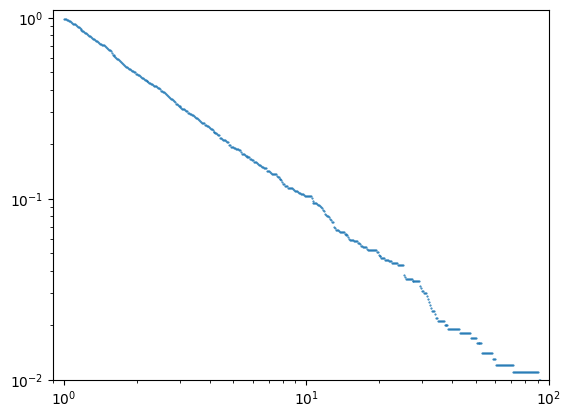

# @title
import matplotlib.pyplot as plt
a= np.array(ag)  # Transformamos a lista em um array
ccfd = []  # Guardaremos as probabilidades
# Vamos definir que valores vamos pegar.
x = np.logspace(-1, 4, 1000)
for i in x:  # Vamos percorrer todos os valores possíveis
    # Quantos agentes tem menos ou igual a i de moedas
    index = np.count_nonzero(a <= i)
    prob = 1-index/(len(ag))  # A probabilidade de alguém ter mais que i
    ccfd.append(prob)  # Salvamos

b = -(np.array(ccfd) == 0).sum() #Plotamos até  ter zero probabilidade
plt.plot(x[:b], ccfd[:b],'o', markersize=0.5)
plt.xscale("log")
plt.yscale("log")
plt.xlim(1E-0,1E1)
plt.ylim(1E-2,1E0)

(0.01, 1.0)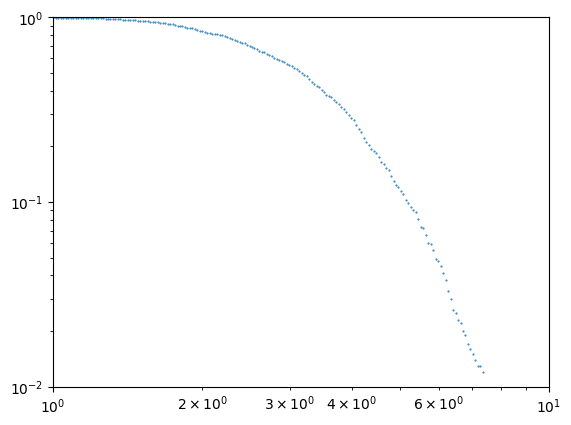

Furthermore, by observing the aggregate wealth distribution of the system—that is, by collecting the wealth $m_{i}$ of all agents at the end of each step of the dynamics—we observe a behavior consistent with a gamma-like distribution in the bulk of the distribution, accompanied by a heavier tail for large wealth values. Although the presence of a power law is not conclusive, the behavior of the tail suggests a possible deviation from simple exponential decay.

# @title
import numpy as np
N=1000 #quantidade de agentes
passos = 10000 #passos de monte carlo
tm = 9000 #A partir de qual passo coletar dados
m = np.array(N*[1.0]) #Dinheiro dos agentes
l= np.random.uniform(0, 1, size=N)

eta = [[] for _ in range(N)]
res=[]  #Os dinheiros de cada agente a cada ano
med=m.copy()  #A riqueza média do agente
ag=[]         #A riqueza um único agente
id=0          #Agente escolhido
c=1           #contador
for t in range(passos):
  # Geramos os lambda e alphas
  a = np.random.uniform(0, 1, size=N)
  a = a / np.sum(a)
  #Copiamos o dinheiro atual
  m0=m.copy()

  #Geramos a fração da riqeuza monetária circulante
  MV=0
  for j in range(N):
      MV+=(1-l[j])*m0[j]

  #Atualizamos o dinheiro atual de cada agente
  for i in range(N):
    m[i]=l[i]*m0[i]+a[i]*MV                      #Artigo 1
    if(t>=tm):
      eta[i].append(MV*a[i])
    #m[i]=l[i]*m0[i]+np.random.normal(0, 0.01)   #Artigo
    #m[i]=l[i]*m0[i]+np.random.exponential(scale=1.0)


  #Então guardamos os dados
  if(t>=tm):
    res.extend(m)
#
    med+=m
    c+=1
    ag.append(m[id])

med=med/c

# @title
import matplotlib.pyplot as plt
a= np.array(res)  # Transformamos a lista em um array
ccfd = []  # Guardaremos as probabilidades
# Vamos definir que valores vamos pegar.
x = np.logspace(-1, 4, 1000)
for i in x:  # Vamos percorrer todos os valores possíveis
    # Quantos agentes tem menos ou igual a i de moedas
    index = np.count_nonzero(a <= i)
    prob = 1-index/(len(a))  # A probabilidade de alguém ter mais que i
    ccfd.append(prob)  # Salvamos

b = -(np.array(ccfd) == 0).sum() #Plotamos até  ter zero probabilidade
plt.plot(x[:b], ccfd[:b],'o', markersize=0.5)
plt.xscale("log")
plt.yscale("log")
plt.xlim(1E-1,2E2)
plt.ylim(1E-2,1E0)

(0.01, 1.0)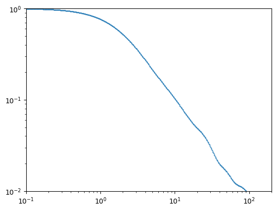

Finally, returning to the model with

\epsilon\left(t\right)=\alpha_{i}(t)\sum_{j}(1-\lambda_{j})m_{j}(t),

(89)

we perform a simple test by drawing each $\lambda_{i}$ from a uniform distribution between 0 and 1. An analogous procedure is applied to $\alpha_{i}$ , with the additional constraint that we normalize it such that $\sum \alpha_{i}=1$ . Then, running a simulation with $N=1000$ agents over 10,000 steps, we collect $\epsilon_{i}\left(t\right)$ from the last 1000 steps.

Considering bins of size $\sqrt{1000}$ , we apply the Ljung–Box test to verify the presence of autocorrelation. The results indicate that in approximately 94% of the cases there is no statistical evidence to reject the null hypothesis of absence of correlation, since the obtained p-values satisfy $p>0.05$ . This behavior is consistent with the 5% significance level adopted in the test, i.e., with the probability of incorrectly rejecting the null hypothesis.

Additionally, computing the mean and standard deviation over each interval for a single agent $i=10$ , we obtain

\frac{\sigma_{\text{media}}}{\mu_{\text{media}}}=0.10 \qquad \frac{\sigma_{\text{desvio}}}{\mu_{\text{desvio}}}=0.09.

(90)

Therefore, in this specific scenario, there is evidence suggesting that $\epsilon\left(t\right)$ can indeed be approximated as white noise. However, not all scenarios were explored, and we did not rigorously test the stationarity of the mean and variance.

# @title
from statsmodels.stats.diagnostic import acorr_ljungbox
janela=int(np.sqrt(len(eta[0])))
# teste de Ljung-Box
c=0;d=0
for e in eta:
  teste = acorr_ljungbox(e, lags=[janela], return_df=True)

  if (teste["lb_pvalue"].iloc[0]>0.05):
    c+=1
    #print("Não há autocorrelação")
  else:
    d+=1
    #print("Há autocorrelação")


medias = []
desvios =[]

for i in range(0, len(eta[0]), janela):

    trecho = eta[10][i:i+janela]

    medias.append(np.mean(trecho))
    desvios.append(np.std(trecho))
print("Razão entre desvio padrão e média da média:",np.std(medias)/np.mean(medias))
print("Razão entre desvio padrão e média do desvio:",np.std(desvios)/np.mean(desvios))

Razão entre desvio padrão e média da média: 0.10060010177488371
Razão entre desvio padrão e média do desvio: 0.08571710106641703

Conclusion¶

The results obtained throughout this work allow for some important conclusions, even though not all possible scenarios have been explored. The discussion developed here reveals certain conceptual difficulties present in attempts to ground econophysics models on marginalist assumptions, especially when one seeks to incorporate elements related to production, savings, interest rates, and monetary circulation without introducing more central mechanisms of capitalist dynamics, such as profit, capital accumulation, effective competition, or private ownership of the means of production. Under these conditions, production essentially functions as a formal mechanism for converting money into commodities, while precisely the elements that characterize the dynamics of capitalism as an economic system remain absent. The introduction of the productive sphere thus ends up being limited to a partial and insufficient formalization.

In the first model analyzed, we observe that the introduction of Cobb–Douglas utility functions and optimization mechanisms under budget constraints leads, after successive simplifications, to the classical kinetic exchange models of monetary transactions. What occurs, therefore, is less a removal of randomness from the model and more a displacement of its formal origin. Randomness no longer appears explicitly as arising directly from wealth transfers, but is instead relocated to the agents’ preferences themselves, whose parameters are assumed to vary randomly at each interaction. However, after successive microeconomic reformulations, the effective dynamics of the system remain essentially governed by stochastic variables of monetary redistribution, and mathematically randomness reappears as the direct regulator of wealth transfers between agents. Thus, rather than a marginalist approach to econophysics, what we obtain is the use of mathematical formalisms to reinterpret randomness in wealth transfers as randomness in the preferences of agent $i$ regarding what agent $j$ has to offer in exchange.

In the generalized model, we must also draw attention to a similar issue. Although we again start from Cobb–Douglas utility functions, optimization mechanisms, and economic considerations (once more omitting central elements) of perfect equilibrium, at a certain point the fraction $\alpha_{i}(t)$ of total social production appropriated by each agent is assumed to be arbitrary. This again leads to a wealth redistribution dynamics whose main mechanism is randomness. If the goal of the model is to ground wealth distribution in a marginalist framework, then the fraction of social product appropriated by each agent cannot remain an essentially arbitrary coefficient.

We thus observe an important methodological tension: although the models initially start from relatively structured economic assumptions, an increasing portion of the dynamics is progressively determined by the statistical properties of the introduced random variables. Ultimately, central aspects of economic dynamics are either ignored from the outset or replaced by stochastic processes without adequate justification.

This does not imply that econophysics models are useless or incorrect. On the contrary, the results obtained show that such models are capable of qualitatively reproducing wealth distributions compatible with several empirically observed patterns, including gamma-like distributions and heavy tails consistent with power laws in certain regimes. However, the results suggest that the most appropriate theoretical framework for grounding and interpreting these models may lie outside the marginalist approach.

The Marxist approach, for instance, by considering that the central element of capitalism lies in the social relations of production rather than merely in technical aspects of circulation or exchange, may offer greater compatibility with highly abstract models of monetary redistribution. Even when a probabilistic approach to the economy is introduced, authors still attempt to provide a justificatory framework for it.

In this sense, it may be methodologically more consistent to abstract entirely from the productive sphere than to introduce its elements only partially while omitting precisely the central mechanisms of capitalist accumulation dynamics.

Thus, the main limitation identified in this work does not seem to lie in the stochastic methods used in econophysics per se, but rather in the attempt to reconcile them with a marginalist microeconomic foundation based on perfect equilibrium assumptions, structurally symmetric agents, and the absence of the central mechanisms of capitalist dynamics.

Note: text translated via ChatGPT.