I don’t want to write too much about this model because I want you to access my paper: Inequality in a model of capitalist economy. Besides that, it is recommended to read:

The social architecture of capitalism: The original paper where the model was proposed (also included in chapter 13 of the book Classical Econophysics).
Agent-Based Models, Macroeconomic Scaling Laws and Sentiment Dynamics: A thesis discussing the model and some modifications.
Implicit Microfoundations for Macroeconomics: A modification proposed by Ian Wright himself.

But I can say that, in general, the central result of this model is that the unequal structure of wealth distribution that emerges in capitalist societies is an intrinsic feature of how capitalism organizes the production and distribution of commodities, and not a punctual failure due to any external reason outside capitalism itself. Given this fact, we have only three options: 1) accept it, 2) try to mitigate it through reforms (e.g., wealth taxes), 3) replace it with a new mode of production.

Abstract by alphaXiv¶

Since I am not interested in producing a very long text, I will take the opportunity to use the summary created automatically by alphaXiv:

Problem¶

Many agent-based models (ABMs) struggle to generate realistic wealth distributions, often resulting in wealth condensation or requiring external interventions like taxes to avoid it.
Existing ABMs frequently rely on exogenously imposed mechanisms (e.g., tax structures, savings propensities) to produce observed economic patterns, making their results dependent on these assumptions.
While Ian Wright’s Social Architecture (SA) model naturally reproduces realistic dual-regime wealth distributions and class structures.

Results¶

The Social Architecture model naturally self-organizes into a distinct two-class society (workers, capitalists) and robustly reproduces dual-regime wealth and income distributions (exponential and power-law) without external interventions.
The dynamics of inequality within the model are primarily governed by a single dimensionless ratio, R = /p (wealth per capita divided by the average wage).
An increase in wealth per capita (analogous to economic growth), while average wages remain fixed, inherently leads to an increase in economic inequality by amplifying wealth concentration among capitalists, challenging the assumption that economic growth benefits all classes equally.

Critical Policy Implications¶

The paper’s most significant contribution lies in its counter-intuitive finding about economic growth and inequality. The analysis demonstrates that “in an economy where total wealth is conserved and with a fixed average wage, the increase in wealth per capita comes with more inequality.”

This challenges conventional wisdom suggesting that overall economic growth (analogous to increasing $\bar{w}$ ) inherently benefits all social classes. Instead, the model shows that growth without corresponding wage increases tends to amplify wealth concentration among capitalists while diminishing workers’ relative economic position.

This finding has profound implications for policy discussions, suggesting that aggregate economic indicators like GDP may be misleading without considering distributional effects. The research supports theoretical arguments that unregulated capitalism has inherent tendencies toward increasing inequality, requiring active policy intervention to achieve more equitable outcomes.

Model¶

The model implemented in this paper is the original SA proposed by Ian Wright. However, we have chosen a slightly different notation and terminology to align with those commonly used in econophysics and agent-based modeling. The society consists of $N$ agents (labeled $i=1,\dots,N$ ), where each agent $i$ has a positive integer quantity $w_i(t)$ representing money which varies over time. An agent is not necessarily an individual, but can represent other economic entities.

The population size $N$ and the total wealth of the system $W= \sum_{i=1}^N w_i(t)$ are conserved, so the wealth per capita $\overline{w}=W/N$ is constant. Agents can be in one of three classes: employees (working class), employers (capitalist class), or unemployed. Then, each agent is characterized by an index $e_i\neq i$ , which identifies their employer: $e_i = j$ if agent $j$ is the employer of agent $i$ , and $e_i = 0$ if agent $i$ is unemployed or employer. Therefore, at any time $t$ , the state of the entire economy is defined by the set of pairs $S(t) = \left\{ \left( w_i(t), e_i(t) \right) :1\leq i\leq N \right\}$ . A firm consists of a set of employees and an employer, which is the only owner of the firm.

In addition to the system size $N$ and the wealth per capita $\overline{w}$ , there are two other parameters: the minimum and maximum wages, $p_a$ and $p_b$ , that each employee can receive. These four are the only parameters of the model. Random selections (of agents, wealth aliquots, wages, etc.) are made uniformly, unless otherwise specified.

In the initial state, all agents have the same wealth ( $w_i(0)={W}/N$ ) and are all unemployed ( $e_i(0)=0$ ). At each time step (which we set to be a month as in the original paper), the following six steps are executed $N$ times, to give each agent the opportunity to be active once per month on average.

Agent selection:

An agent $i$ is randomly selected.

Then, the following rules are applied, being 3, 4 and 6 related to wealth exchanges, while rules 2 and 5 are related to changes of status.

Hiring Only if $i$ is unemployed, then:

A potential employer $j$ is selected from the set $H$ of all agents except the employees, with probability $P (j)= w_{j}/\sum_{n\in H}w_{n}$ .
If $w_j \ge \overline{p}$ (average of the distribution from which the wage is drawn), then: the agent $i$ is hired by $j$ . Hence $j$ becomes an employer if it was previously unemployed.

Expenditure (on goods and services):

A random integer $w$ in the range $\left[0,w_{k}\right]$ is selected for a random agent $k\neq i$ . Then, the following transfer to the market value $V$ occurs:

\notag w_k \to w_k-w, \quad V \to V+w.

(1)

Market revenue (from sales of goods and services):

Only if $i$ is not unemployed, the following transfer from the market value occurs:

\begin{align*} \notag && \;\;\;\;\;V \to V-w, \\ \notag % && \begin{cases} w_i\to w_i+w , &\mbox{if $i$ is employer,}\\ w_{e_i}\to w_{e_i}+w , &\mbox{if $i$ is employee,} \end{cases} \end{align*}

(2)

where $w$ is a random integer number $w\in \left[0,V\right]$ . In all cases, the quantity $w$ is counted as firm revenue $r_i$ .

Firing Only if $i$ is an employer, then:

The number $m$ of employees to be fired is defined according to the formula $m=max(n_{i}-\frac{w_{i}}{\overline{p}},0)$ , where $n_i$ is the number of employees of agent $i$ .
A number $m$ of agents from the list of $i$ ’s employees are randomly selected to be fired. -Furthermore, if all the workers are fired, then the employer $i$ becomes an unemployed.

Wage payment Apply only when agent $i$ is an employer. For each agent $j$ employed by $i$ , the following transfer occurs

\notag w_i \to w_i-p, \quad w_j \to w_j+p.

(3)

where $p$ is a discrete amount randomly selected from the interval $[p_a,p_b]$ , but if $p > w_i$ , then a new wage $p$ is selected from the interval $[0,w_i]$ .

Main results¶

I will summarise the paper’s main results here.

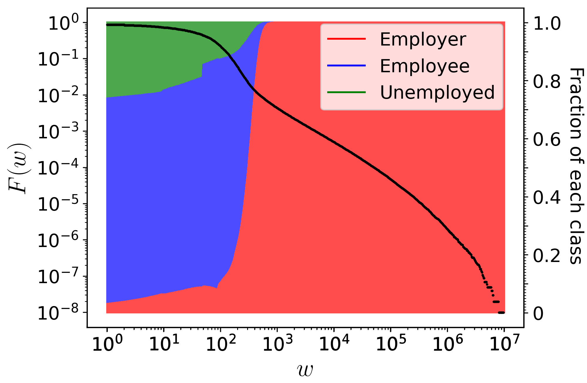
This graph shows the complementary cumulative distribution fuction (CCDF) of wealth, as well as its social composition. We can observe that up to approximately 10³ coins, capitalists make up less than 10% of the agents holding such wealth. The vast majority of agents with wealth between 0 and 10³ are employees or unemployed.

Above this threshold, the probability of finding an agent with that level of wealth decreases sharply, until only a small fraction concentrates amounts on the order of up to 10⁵ coins. Considering that this simulation involved approximately 10⁵ agents and an average wealth of 100 coins per capita, the total wealth in the system is about 10⁷ coins. This implies that, in the extreme, a single capitalist is capable of concentrating virtually all the available wealth.

This also becomes evident when we separate wealth by class. Above 10³ coins, there is basically no possibility of finding an agent who does not belong to the capitalist class. Conversely, practically 100% of capitalists hold a wealth of at least 10².

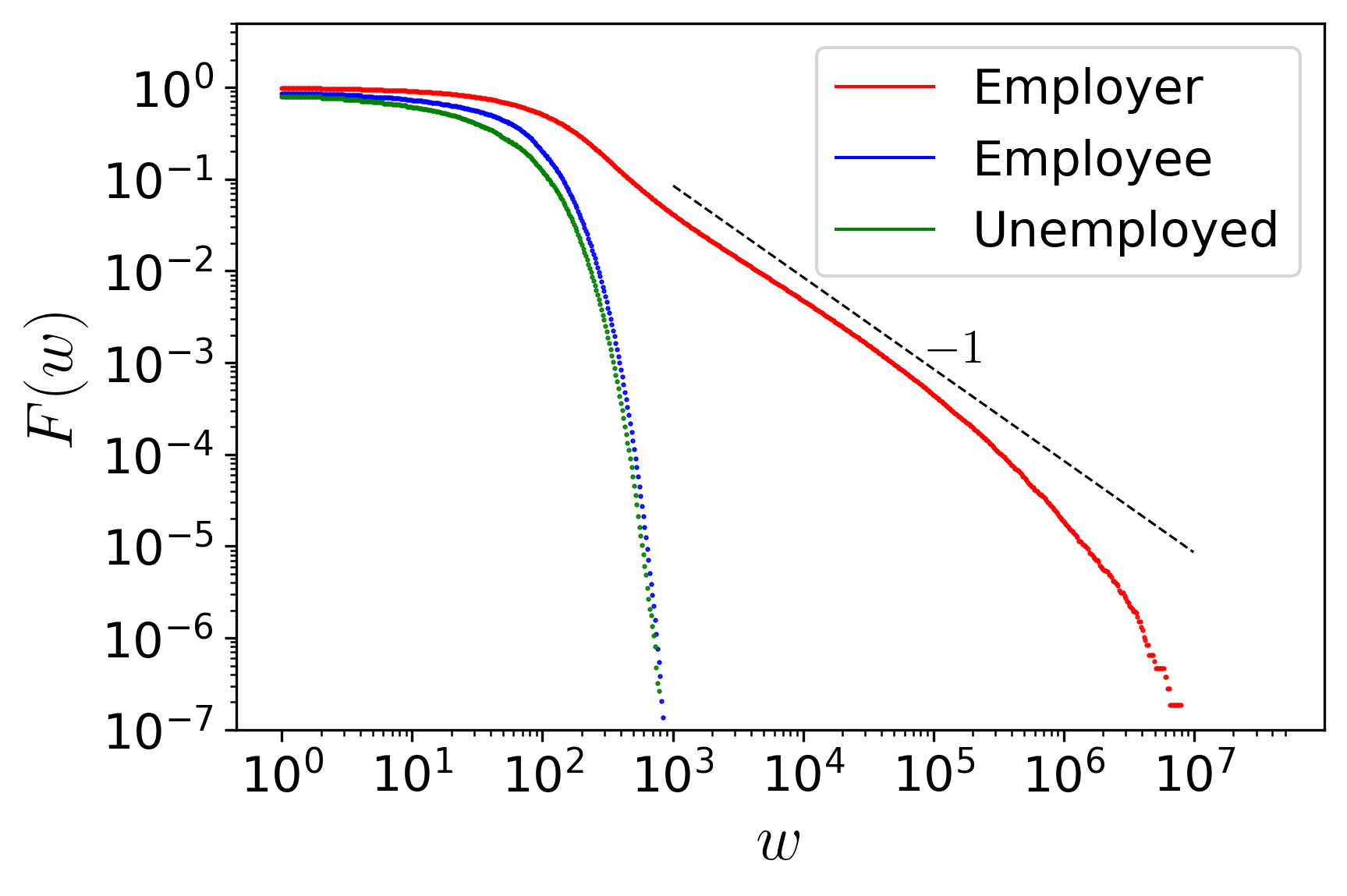
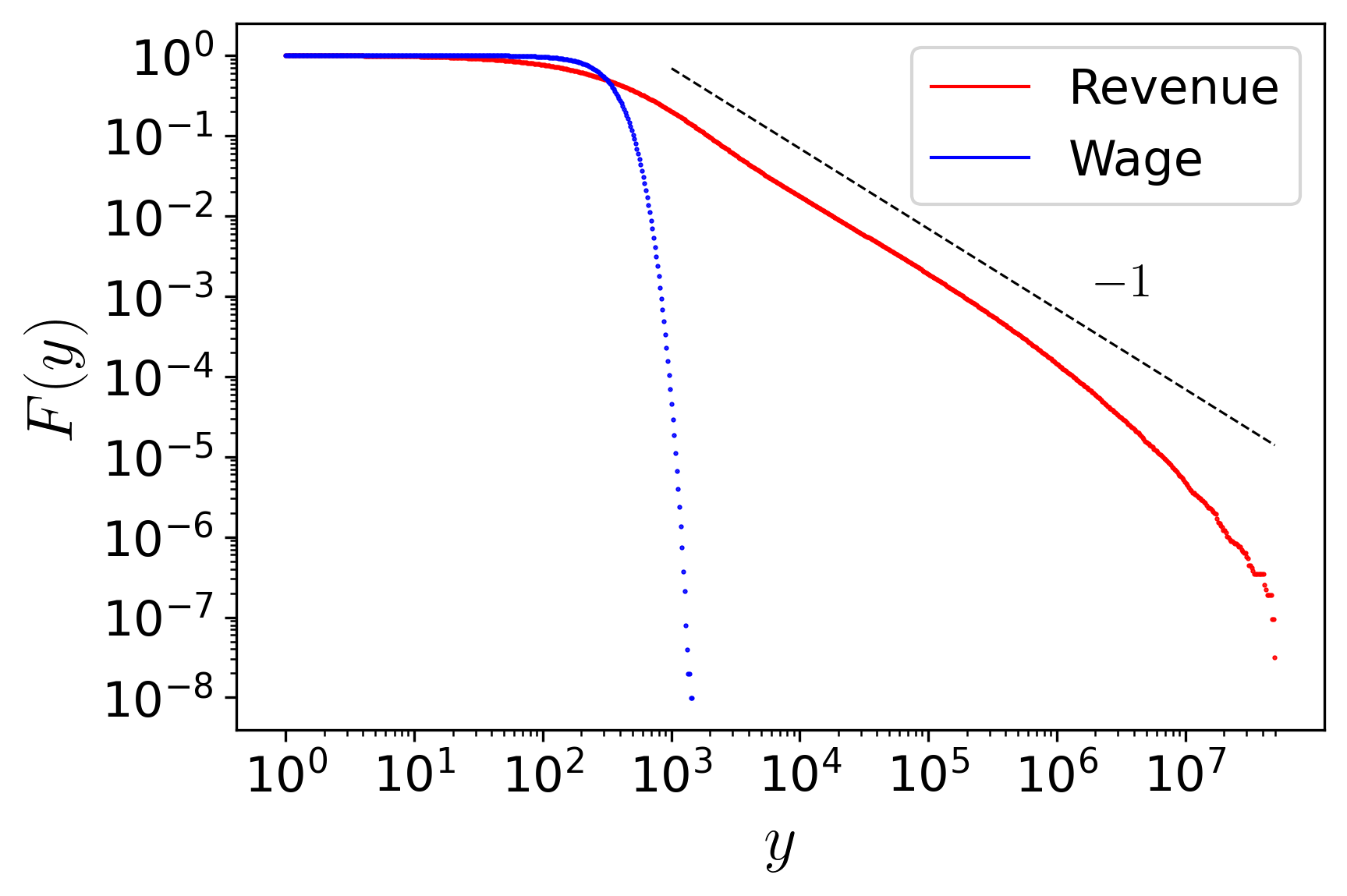
The income distribution follows a pattern similar to wealth. When we distinguish between the source of income (revenue as a firm owner, or wage as an employee), we can notice that the pattern repeats. All these results are consistent with real-world data, which point to the existence of two regimes in the wealth distribution of society: an exponential distribution (Boltzmann-Gibbs-like) for the majority of the population with lower income, and a power-law distribution (Pareto-like) for the small fraction of the super-rich population with higher income.

It is also important to mention that the main result obtained by the model is that the only relevant parameter of the model is the parameter ( $R=\left\langle w\right\rangle /\left\langle p\right\rangle\$ ), given by the ratio between per capita wealth ( $\left\langle w\right\rangle\$ ) and the average wage ( $\left\langle p\right\rangle\$ ). In other words, as long as the ratio is respected, it does not matter whether we increase per capita wealth or decrease the average wage. The result can be seen in the figure below where we increase per capita wealth:

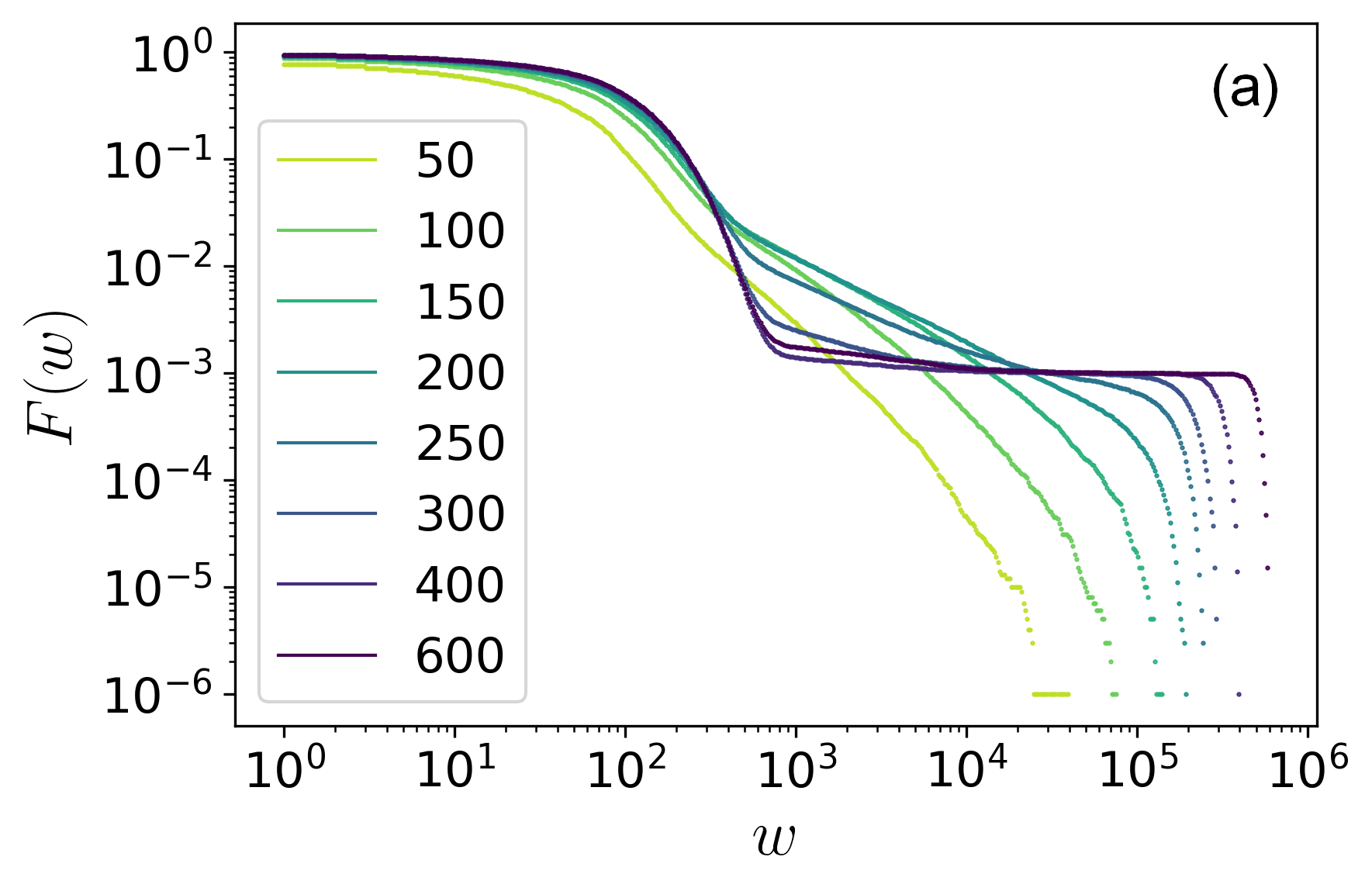
What can be noticed is that inequality increases, something that can be verified through the change in the Gini coefficient, as seen below:

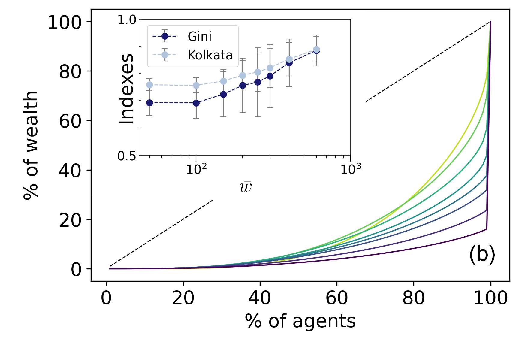
By combining these results, we can make two statements: a) The model satisfactorily captures the division into two classes of wealth (and income) presented by capitalist economies. b) In this model, increasing total wealth does not translate into benefits for workers; on the contrary, it deepens inequality. We can conclude by highlighting that the model shows that inequality is an intrinsic feature of capitalism—it is how it functions, not a flaw. One suggestion that the model makes is that the improvement of workers’ living conditions occurs through political struggle, not as a mere technical consequence.

Expanded Discussion¶

I want to delve a bit deeper into the discussion of this model and its results, based on Chapter 10 of the book Classical Econophysics, the first place where I had access to Wright’s model of the social architecture of capitalism. In the book, it is also referred to as the “probabilistic model of the social relations of capitalism.”

The dominant social relations of production in capitalism are between capitalists and workers. A small class of capitalists employs a large number of workers organized in firms of various sizes to produce goods and services to be sold on the market. Under normal circumstances, the capitalist collects the revenue, and the workers receive a portion of it in the form of wages.

Over the past century or more, the number and type of goods and services offered by capitalist economies have changed, but the social relations of production have not. The existence of social relations between the capitalist class and the working class, mediated by wages and profits, is an invariant feature of capitalism.

Many economic models describe utility relations among economic agents and the type of scarce commodities, or theorize about the material-technical dependencies between inputs and outputs in the production process. But what we want to examine are the social relations of dependency mediated by money. As such, the model is constructed solely from money and agents. The idea is to focus as much as possible on the economic consequences of the social relations of production—that is, on the social architecture—rather than any particular or even transient mechanism, such as a specific market or commodity. Since the worker-capitalist relation is the dominant social relation in capitalism, the model abstracts away from land, the state, banks, and other factors.

We then build a computational model of the social architecture of capitalism. Although we use a small and simple set of hypotheses about relations in capitalism, when we simulate it, we can observe that it replicates some of the most important characteristics of modern capitalism. The computer thus serves as a logical testing ground, and the simulation allows us to explore the complex consequences of our simple assumptions. It lets us determine whether important large-scale features of a capitalist economy necessarily arise from its most basic social relations.

The features of capitalism that the article aimed to recreate are:

The structural division of society with a small number of employers and a large number of employees.
The distribution of income by class and individual.
The distribution of firms into a small number of large companies (both by size and capital) and a large number of small companies.
The way in which firm growth clusters around the average growth.
The way in which firms die.
The distribution of GDP growth rates and recessions.

For each of these criteria, the goal is to examine the predicted statistical structures obtained from the computational model and compare them with what is known about the statistical properties of corresponding real-world data. The objective is to see whether a formal model of the social relations of capitalism can predict what we know about the statistical properties of capitalist economies.

In this way, we can begin to understand which characteristics of capitalism are necessarily consequences of how the economy is socially organized. For example, we can see that extreme income and wealth inequality appears to be a necessary feature of capitalist social relations.

This does not imply that we need to accept it; there are many political responses to this scientific fact: accepting its necessity (pro-capitalism), trying to alleviate it within the current social relations (reformism), or accepting the need to change the social relations (anti-capitalism). However, regardless of the preferred political response, the economic model we develop indicates that there are powerful and enduring market forces that continuously generate inequality, independent of the subjective intentions of politicians.

Model¶

One warning: since the model considers a purely capitalist economy, with the assumption of a finite set of agents, it proposes a situation that differs from Marx’s assumption of the existence of a latent reserve army of potential workers in non-capitalist sectors who could enter the capitalist sector and regulate wages. It should also be noted, however, that the number of agents is fixed, this can be interpreted as a stable workforce, where entry and exit occur at the same rate.

Labor Market

The labor market is modeled in a simple way: all unemployed agents want to be employed, and employers hire if they have sufficient funds to pay the average wage. Anyone who is not a worker can then become an employer, but the odds favor those who possess greater wealth.

Spending on Goods and Services

Each agent spends their income on goods and services. Spending in particular is not modeled in detail, but aggregated into a single quantity representing the agent’s total expenditure. Total expenditure can represent multiple small purchases, one large purchase, or installments of a purchase; the interpretation is intentionally quite flexible. Without inserting a theory of consumption patterns, the only relevant information is that an agent’s spending is limited by how much money they have.

This rule governs the spending of all consumers, whether capitalists, workers, or unemployed. Clearly, the wealthy have a greater chance of spending more. Different classes have different spending patterns: while workers typically spend their income on goods, capitalists also invest. Wages are treated separately, so salaries are not considered expenditures. It is assumed that there is an implicit saving rule, as the probability of an agent spending everything at once is low.

Interaction Between Firms and the Market

To simplify, we assume that all means of production belong to capitalists and individual agents are unable to produce. This model also ignores self-employment. Productive work results in goods and services that can be sold, performed only by agents within firms.

The types of commodities and individual sales are not modeled; instead, only the transfer of money from the market to the seller is modeled, represented as several separate transactions or fractions of a single large transaction.

Under normal circumstances, a firm expects that the value added by a worker to the product is at least equal to the worker’s wage. After all, if the value added by the worker is less than the salary paid, the firm would incur a loss; it would be more advantageous to sell the product without any added value. A firm’s profit margin over costs reflects this expectation, which may or may not be validated by the market. Naturally, various factors can cause a worker to add more or less value to the final product, which is difficult to measure and partially reflected in the wide range of negotiable compensation.

We model the concrete relationship between labor and added value by assuming that the firm randomly draws a sample of market value once per month for each employee. Samples per employee reflect the fact that each worker potentially adds value, but the randomness of each sample reflects the variety of possibilities, from irreplaceable movie stars to easily replaceable administrators. This is a weak formulation of the labor theory of value, which implies that, in the absence of a profit-equalizing mechanism, there is a statistical tendency for a firm’s product value to be linearly related to the amount of socially necessary labor time spent on it, and consequently, the greater the number of employees in a firm, the higher its profit.

Thus, each firm draws a market sample to earn revenue for each employed worker. In an idealized competitive economy, there is a tendency for productions with particular advantages to be adopted by competing firms, including the elimination of scarcity due to the use of specialized labor in particular tasks. We can then assume that the value added per worker is statistically uniform across firms. Statistical variation can be interpreted as representing transient differences in the productivity of different concrete jobs.

Even though different workers may be more or less productive, the value obtained from their work is constrained by the average level of market demand. The value added by an active worker to a firm’s product is represented by a transfer of money from the current market.

The actual value received in monetary form depends on market conditions; the relationship between costs and revenue determines whether firms are rewarded with profit for performing socially necessary work. The profit received from the market is the legal property of the capitalist who owns the firm. In this way, firm owners accumulate revenue through market sales that represent the social utility of their workers’ efforts.

We model it such that the contributions of employee and employer are the same. Of course, we are only talking about expected value; the individual contributions of agents will vary randomly. In a real economy, high motivation may allow employers to contribute more per day than employees, but we ignore this for simplicity.

The money received may represent the embedded value of many types of products and services sold in arbitrary quantities to arbitrary numbers of buyers. The market sampling rule abstracts away from these individual transaction details and can be interpreted as modeling the aggregated effect of the dynamics of a random graph connecting buyers and sellers in each period.

Labor and Wages

In this model, there are no skill differences between agents. Therefore, it does not matter which agent is employed, only the quantity. A new firm is formed when two agents enter an employer-employee relationship, and existing firms may cease to exist if all employees are dismissed and the owner becomes unemployed.

There is also no difference in agents’ wages; they are drawn from a uniform distribution. In reality, wages are not subject to stochastic fluctuations; a more elaborate model could introduce wage contracts between agents that fix the wage for a certain duration. However, in the total sum, in terms of total company expenditures or the national income distribution, the existence of individual wage fluctuations is not significant and allows for considerable simplification.

The “monthly rule” implies that each month, a set of rules is executed N times to allow the N agents the opportunity to act. Of course, this does not guarantee that all actors will necessarily act in the month; some may act more than once, while others may not act at all. This introduces a level of intentional randomness to model the fact that in real economies, events do not occur with strict regularity. Logically, a year is defined as 12 applications of the monthly rule. The model thus provides a time scale linked to real time by the fact that, on average, wages are paid monthly.

Results¶

Over the past 20 years, it has become clear that very simple computational models can generate complex behaviors. Key results:

The current amount of money M and the number of agents N act as scaling parameters and do not affect the dynamics.
The size of the wage range does not affect the dynamics.
If we increase M and N proportionally, wealth per agent remains the same.
If we increase M alone, average wealth $\overline{w}$ increases. So the parameter defined as $R=\overline{w}/ \overline{p}$ increases, and inequality also rises.
If the number of agents is very small, the model behaves qualitatively differently. However, real economies are composed of millions of people.
Changing the average wage $\overline{p}$ affects the emerging dynamics. Keeping per capita wealth constant, we decrease $R$ and reduce inequality.

Among the main results, as previously noted, is the division of national wealth into two classes—a result that seems to agree with the predictions of Farjoun and Machover.

At the start of the simulation, the system quickly organizes into a static equilibrium. In this equilibrium, individual agents’ wealth fluctuates, but the probability distribution does not fluctuate over time. The simulation does not reach a motionless equilibrium, but rather converges to a dynamic equilibrium with continuous movement and changes.

Moreover, the stratification generated in capitalist economies is a complex phenomenon related to the dominant social relations of production. In reality, the social relations of production are much more complex than those presented in this model, but it is evident that the capitalist class is numerically small compared to the working class. In other words, those who rely on wages for subsistence constitute the large majority of the population; this model also successfully captures this fact.

The full results obtained through this model can be found in the papers presented at the beginning of the text. However, it can be said that the empirical coverage of the model is extensive, even though the model was defined from small and simple economic rules governing the dynamics. The model compresses and connects a large amount of empirical data within a single framework. The idea was to show how the peculiar social relations of capitalism have a pervasive effect and determine many of the properties of capitalism at a macro level. We can extend this modeling in many ways and explore many aspects that can be measured and analyzed; this is just a starting point.

In this system, we move from micro-economic social relations to the emergent macro-economic phenomenon. However, why a set of rules necessarily generates dynamics observed as a consequence can be initially difficult to understand. This is why computational modeling is not an alternative to mathematical deduction, but connected to it.

Within the explored parameter space, the model generates fluctuations in national income around long-term stable averages. However, a deeper study is necessary to understand why this occurs. The computational model demonstrates that, in principle, if a deduction can be produced, its basic assumptions will correspond to those of the computational model, but of course, a deductive proof may be more or less difficult to obtain.

Thus, the use of computational modeling makes it easier to identify theories that can then be analyzed to generate explanations in the form of mathematical deductions or natural language explanations, aiming to gain a deeper understanding of the dynamics of the analyzed system. A purely deductive approach, where the investigator can explore only candidate theories that are directly accessible to a mathematical deduction, is unnecessarily restrictive, particularly if the system presents analytical challenges.

The basic elements of this model therefore differ from standard economic models. For example, standard competitive or neoclassical equilibrium models typically start from an ontology of rational agents who maximize self-interest in a scarce resource market: the focus is on determining the equilibrium exchange rate of commodities, which is a solution to a set of static constants. Typically, money is not modeled, and time is absent.

Neo-Ricardian models, on the other hand, start from the ontology of production technique relations between different types of commodities, which define the material transformation available for agents to perform. The production of commodities results in a surplus that is distributed between capitalists and workers. Despite differences between the models, there are similarities. Prices in these models are also exchange rates determined by solutions conditioned on constants, and time is also absent. There is also no explanation of why or how a particular configuration of the economy produces effects.

There is a difference between these models and the one developed here. The most obvious is that we have neither types of commodities nor rational agents. Instead, we model the elements of the economy that are ignored in these other models, specifically the agent-to-agent relationships mediated by money that occur over time. At an abstract level, neoclassical models theorize scarcity constraints and neo-Ricardian models production-technical constraints; this model theorizes the dynamic consequences of social constraints, which are historical facts about how economic production is socially organized.

There are deep sociological reasons why standard economic theory is resistant to criticism and has remained largely unchanged. Furthermore, the model we describe here provides proof that the standard ontology is redundant for forming explanations of the phenomena it aims to explore.

It does not deny that other issues may require considering the purposefulness of activity for explanation, and thus the introduction of rational agents or consideration of production-technical constraints, and then the introduction of types of commodities. What the model described here claims is that, for the empirical aggregates considered, there is no need to reduce political economy to psychology and technical production conditions, and that the dominant causal factors are not found at the individual behavior level, nor at the level of production-technical constraints, but are found at the social level of production relations, which constitute an abstract, yet no less real, social architecture that constrains the actions individuals can take, whether optimized or not.

This is why agents choose among possible economic options restricted by their class and the money they possess. This is an approximation to the classical political economy conception of Smith, Ricardo, and Marx, in which individuals are considered representatives of economic classes that have defined relations with each other in the production process. The social architecture—particularly the social relation of wage-capital—dominates individuals, who in turn are free to make local economic decisions, but within a social environment that is not under their control.

The method of abstraction of rationality adopted here, rather than emphasizing the particular nature of individuals, is valid because the number of degrees of freedom that the economic reality presents is very large. This allows the rationality of individuals to be modeled with a highly stochastic selection from a set of possibilities defined according to the social architecture.

The quasi-psychological motives that supposedly guide individual actions can be ignored in this approach because, within a large set of individuals, they rarely matter.

Final Considerations

Our goal was to begin understanding the economic consequences of social relations of production and to develop a model that included money and time among the essential elements. The motivation for this approach is based on Marx’s distinction between invariant social relations of production and the variable forces of production. Capitalism changes over time, but the existence of the social roles of worker and capitalist is unaltered and an intrinsic characteristic of it.

The production model replicated some important empirical features of modern capitalism:

The tendency of capital concentration resulting in a highly unequal distribution characterized by a lognormal distribution with a “Pareto tail”
The Zipf or power-law distribution of firm sizes
The Laplace distribution of firm sizes and GDP growth
The exponential distribution of recession durations
The lognormal distribution of firm exits
The Gamma-type distribution of profit rates

The model also naturally generates groups of capitalists, employees, and unemployed in realistic proportions, as well as the business cycle phenomenon, including fluctuating wages, profits, and the division of national income.

The good qualitative—and in many cases quantitative—agreement between the model and empirical phenomena suggests that the theory presented here captures some essential characteristics of the capitalist economy, and demonstrates the importance of social relations of production, as well as serving as a foundation for more concrete and elaborated models.

A final conclusion we can draw is that the implication that certain features of the economy that cause political conflicts, such as income inequality and recessions, are necessary consequences of the social relations of production, and therefore essential properties of capitalism, not merely accidental, transient, or exogenous events.

Codes¶

I was going to write the code in Python, but since I already have it in C#, I’ll share it in C# for now.


// Names of variables translated via ChatGPT

using System;
using System.Collections.Generic; // Lists
using System.IO;                  // File
using System.Text;                // Use of StringBuilder

namespace HelloWorld
{
    class Program
    {
        static void Main()
        {
            // System parameters and variables

            for (int ii = 0; ii < 10; ii++)
            {
                int numAgents = 1000;                         // Number of agents
                int initialMoney = 100;                        // Initial money
                int years = 1000;                              // Duration of simulation in years
                int maxSteps = years * 12 * numAgents;         // Duration in steps
                var agents = new int[numAgents + 1];           // i -> index, j -> value. j is the boss of i, -1: employer, 0: unemployed, j: employee of j
                var wealth = new int[numAgents + 1];           // Wealth list
                var salaries = new int[numAgents + 1];         // Income list
                var profits = new int[numAgents + 1];          // Profit list
                List<int> employers = new List<int>();          // List of employers
                List<int> unemployed = new List<int>();         // List of unemployed agents
                int minSalary = 10;                             // Minimum wage
                int maxSalary = 90;                             // Maximum wage
                int avgSalary = (minSalary + maxSalary) / 2;   // Average wage
                int seed = ii;

                // Random generator
                Random rnd = new Random(seed);

                // For results analysis
                int currentYear = 0;
                StringBuilder textOutput = new StringBuilder(); // Text to be written
                StringBuilder fileName = new StringBuilder();   // File name
                fileName.AppendFormat("{0:d}-{1:d}-{2:d}-{3:d}-{4:d}.txt", numAgents, initialMoney, minSalary, maxSalary, seed);

                // Initial wealth distribution and connections
                for (int i = 1; i <= numAgents; i++)
                {
                    wealth[i] = initialMoney;        // Assign initial wealth to agent i
                    agents[i] = 0;                   // All agents start without relations
                    unemployed.Add(i);               // All agents start unemployed
                }
                wealth[0] = 0;                       // Market wealth

                // Simulation loop
                for (int i = 0; i < maxSteps; i++)
                {
                    int a, b; // Active agent (a) and interacting agent (b)

                    // 1 - Selection
                    a = rnd.Next(numAgents) + 1; // Ignore agent 0 (market)

                    // 2 - Hiring
                    if (agents[a] == 0) // If a is unemployed
                    {
                        if (employers.Count > 0 || (unemployed.Count > 1))
                        {
                            b = a;
                            bool continueHiring = true;
                            while (b == a)
                            {
                                List<int> empWealthCum = new List<int>();
                                List<int> unempWealthCum = new List<int>();
                                int totalUnemp = 0, totalEmp = 0;

                                for (int j = 0; j < unemployed.Count; j++)
                                {
                                    totalUnemp += wealth[unemployed[j]];
                                    unempWealthCum.Add(totalUnemp);
                                }
                                for (int j = 0; j < employers.Count; j++)
                                {
                                    totalEmp += wealth[employers[j]];
                                    empWealthCum.Add(totalEmp);
                                }

                                if (totalUnemp + totalEmp == 0)
                                { break; }

                                else if (rnd.Next(1, totalUnemp + totalEmp + 1) <= totalEmp)
                                {
                                    int k = rnd.Next(1, totalEmp + 1);
                                    for (int j = 0; j < empWealthCum.Count; j++)
                                    {
                                        if (k <= empWealthCum[j])
                                        {
                                            b = employers[j];
                                            break;
                                        }
                                    }
                                }
                                else
                                {
                                    if (totalUnemp + totalEmp == wealth[a]) { continueHiring = false; Console.WriteLine("Oops!"); break; }

                                    int k = rnd.Next(1, totalUnemp + 1);
                                    for (int j = 0; j < unempWealthCum.Count; j++)
                                    {
                                        if (k <= unempWealthCum[j])
                                        {
                                            b = unemployed[j];
                                            break;
                                        }
                                    }
                                }
                            }

                            if (avgSalary <= wealth[b] && continueHiring)
                            {
                                agents[a] = b;
                                unemployed.Remove(a);
                                if (agents[b] != -1)
                                {
                                    unemployed.Remove(b);
                                    employers.Add(b);
                                    agents[b] = -1;
                                }
                            }
                        }
                    }

                    // 3 - Spending
                    b = a;
                    while (b == a) { b = rnd.Next(numAgents) + 1; }
                    int moneySpent = rnd.Next(wealth[b] + 1);
                    wealth[0] += moneySpent;
                    wealth[b] -= moneySpent;

                    // 4 - Firms
                    if (agents[a] != 0)
                    {
                        moneySpent = rnd.Next(wealth[0] + 1);
                        wealth[0] -= moneySpent;

                        if (agents[a] > 0)
                        {
                            b = agents[a]; // Employer index
                            wealth[b] += moneySpent;
                            profits[b] += moneySpent;
                        }
                        else if (agents[a] < 0)
                        {
                            wealth[a] += moneySpent;
                            profits[a] += moneySpent;
                        }
                        else { Console.WriteLine("Should not enter here"); }
                    }

                    // 5 - Firing
                    if (agents[a] == -1)
                    {
                        int numToFire = 0;
                        List<int> employeesList = new List<int>();
                        for (int j = 1; j <= numAgents; j++) { if (agents[j] == a) { employeesList.Add(j); } }
                        while ((employeesList.Count - numToFire) * avgSalary > wealth[a]) { numToFire += 1; }
                        while (numToFire > 0)
                        {
                            b = rnd.Next(employeesList.Count);
                            int worker = employeesList[b];
                            unemployed.Add(worker);
                            employeesList.Remove(worker);
                            agents[worker] = 0;
                            numToFire -= 1;
                        }

                        if (employeesList.Count == 0)
                        {
                            employers.Remove(a);
                            unemployed.Add(a);
                            agents[a] = 0;
                        }
                        else
                        {
                            // 6 - Wages
                            for (int j = 0; j < employeesList.Count; j++)
                            {
                                b = employeesList[j];
                                moneySpent = rnd.Next(minSalary, maxSalary + 1);
                                moneySpent = (moneySpent <= wealth[a]) ? moneySpent : rnd.Next(wealth[a] + 1);
                                wealth[b] += moneySpent;
                                salaries[b] += moneySpent;
                                wealth[a] -= moneySpent;
                            }
                        }
                    }

                    // Annual data collection
                    if ((i + 1) % (12 * numAgents) == 0)
                    {
                        currentYear += 1;
                        textOutput.Clear();
                        for (int j = 1; j <= numAgents; j++)
                        {
                            textOutput.AppendFormat("{0:d} {1:d} {2:d} {3:d} {4:d} {5:d}\n", wealth[j], agents[j], currentYear, salaries[j], profits[j], j);
                            salaries[j] = 0;
                            profits[j] = 0;
                        }
                        File.AppendAllText(fileName.ToString(), textOutput.ToString());
                    }
                }
            }
        }
    }
}

I recently saw that the second rule in particular can be written more efficiently, since we can replace the two lists (employers and unemployed) with just one list of potential employers. I also received a suggestion to use tuples to store each agent’s information. While I updated the first improvement in my private code (I should update this page at some point), I haven’t implemented the second improvement yet.

I am also sharing a simple Python code to visualize the complementary cumulative distribution function (CCDF) of wealth and income.

# -*- coding: utf-8 -*-
import matplotlib.pyplot as plt
import numpy as np
import locale

# Set locale to Brazilian Portuguese (uses comma as decimal)
locale.setlocale(locale.LC_NUMERIC, "pt_BR.UTF-8")


M = ["List_of_files_to_be_read.txt"]

lists = []

start_year = 1000
end_year = 2000

for N in M:
    f = open(N, "r")  # Open the file
    line = f.readline()
    data_list = []

    while (line != ""):
        data = line.split()
        if (int(data[2]) > end_year):
            print("pause")
            break
        elif (int(data[2]) > start_year):
            #value = float(locale.atof(data[0]))                               # Wealth
            value = float(locale.atof(data[3])) + float(locale.atof(data[4]))  # Income
            data_list.append(value)
        line = f.readline()
    #data_list = [x for x in data_list if x != 0]  # Clean the vector, remove zeros
    data_list.sort()
    lists.append(data_list)
    f.close()

plots = []
for data_list in lists:
    a = np.array(data_list)   # Convert the list to an array
    ccdf = []                 # Will store probabilities

    # Define the values we will use. Here we will count between 0 and val[0], val[0] and val[1], etc...
    lim = 10
    pts = 1000
    x = np.logspace(0, lim, pts)

    for i in x:  # Loop over all possible values
        # How many agents have less than or equal to i coins
        index = np.count_nonzero(a <= i)
        prob = 1 - index / (len(data_list))  # Probability of someone having more than i
        ccdf.append(prob)                    # Save it
    plots.append(ccdf)


fig, ax = plt.subplots()
for ccdf in plots:
    b = -(np.array(ccdf) == 0).sum() # Plot until probability is zero
    plt.plot(x[:b], ccdf[:b])

ax.set_xscale("log")
ax.set_yscale("log")
plt.show()
plt.close()

Below is an example of code that generates the Lorenz curves and calculates the Gini coefficient.

# -*- coding: utf-8 -*-
import numpy as np
import locale
import matplotlib.pyplot as plt
locale.setlocale(locale.LC_NUMERIC, "pt_BR.UTF-8")

# READ THE FILES ----------------------------------------------------------------------
M = ["List_of_files_to_be_read.txt"]
Nagents = 1000                       # Number of agents
Gm = []
Gd = []
ys=[]
lists = []

for N in M:
    f = open(N, "r")                  # Open the file
    line = f.readline()               # Read the file
    ginis = []
    year = Nagents * [0]
    j = 0                             # Index of the agent whose data will be stored
    data_list = []
    while (line != ""):
        data = line.split()
        year[j] = float(locale.atof(data[3])) + float(locale.atof(data[4]))    # Income
        #year[j] = float(locale.atof(data[0]))                                 # Wealth
        if ((j + 1) != Nagents):             # If the next one did not switch to a new year
            j += 1                           # Move to the next agent
        else:                                # If switched to a new year
            j = 0                            # Reset the agent index
            year.sort()                      # Reorganize all agents for the current year
            y = 100 * [0]                    # Create the vector to calculate the Gini coefficient
            x = [i for i in range(1, 101)]   # The x-axis (percentiles)
            current = 0                      # Current percentile
            one_percent = int((len(year)) / 100)   # 1% of the population
            total = sum(year)                # Total income (or wealth)
            share = 0                        # Cumulative income share for the current percentile
            for i in range(len(year)):       # Iterate through all possible values
                share += year[i] / total     # Add normalized income share
                if ((i + 1) % one_percent == 0):   # Every time 1% of population is reached
                    y[current] = 100 * share  # Convert to percentage
                    current += 1             # Move to the next percentile
            y[-1] = 100                      # The entire population owns 100% of the wealth.
            T = sum(x)                       # Total area
            B = sum(y)                       # Area below the Lorenz curve
            A = T - B                        # Area above the Lorenz curve
            gini = A / T                     # Current Gini coefficient
            ginis.append(gini)               # Save Gini
            year = Nagents * [0]             # Move to next year
            ys.append(y)
        line = f.readline()
    Gm.append(np.array(ginis).mean())
    Gd.append(np.array(ginis).std())

for k in range(len(Gm)):
    print("Gini coefficient: {:.2f}±{:.2f}".format(Gm[k], Gd[k]))
    plt.plot(x,ys[k])
plt.plot(x,x,'k')